OCS Research Paper · Preprint · Paper F (the accretion limit)
A Joint Radio–Infrared–X-ray Bound on Bondi-fed Accretion onto the Candidate Intermediate-Mass Black Hole in Omega Centauri
v2.1, last revised 2026-09-03 · Paper F of eight (A: hypothesis · B: review · C: observational campaign · D: economics · E: engineering and adjudication · G: X-ray census · H: mass tension · AXI: methods companion to H)
Three deep non-detections now constrain any accretion flow onto the candidate intermediate-mass black hole (IMBH) at the center of Omega Centauri: a 170-hour ATCA radio campaign reaching 1.1 μJy rms at 7.25 GHz (Mahida et al. 2026), JWST NIRCam/MIRI imaging showing no accretion-like point source at any proposed center (Chen et al. 2025), and a 291-ks Chandra exposure bounding LX(0.5–7 keV) ≤ 1.6×1030 erg s−1 (Haggard et al. 2013). Chen et al. (2025) compare the infrared and radio limits qualitatively; no formal joint bound with propagated uncertainties has been published. We supply one, as a posterior. Defining the Bondi radiative efficiency εB ≡ Lbol/(ṀBc2), we build a forward model from (εB, M) and eight shared nuisance parameters (gas density, sound speed, distance, two SED band fractions, fundamental-plane scatter as a latent variable, inflow-suppression index, electron-heating fraction) to the three measured quantities, evaluate Gaussian likelihoods on the measurements themselves, and report the 95 per cent credible upper limit ε95(M) for three named accretion-flow families. For a radiatively inefficient (RIAF-like) flow, ε95 = 2.9×10⁻¹⁰ at the fast-star mass anchor of 8,200 M☉ and 1.1×10⁻¹¹ at 4×10⁴ M☉; removing the fundamental-plane radio leg entirely relaxes these to 1.4×10⁻⁸ and 7.9×10⁻¹⁰. Overplotting the expectation band for a natural outflow-suppressed hot flow at the same nuisance draws converts the curve into a calibrated verdict. Scoring each natural-flow draw against the measured data directly, the data reject 85 per cent of that parameter space at the fast-star anchor, 78 per cent at the pulsar-timing point-mass cap and 99 per cent at 4×10⁴ M☉ (28, 20 and 76 per cent using no radio information). A Bondi-fed hot flow at a 47 Tucanae-like density is therefore disfavoured across the contested mass range rather than only at its top, and something must give at every anchor: the mass, the gas density, or the suppression physics. Two of those figures replace weaker ones from earlier drafts of this paper, which reported 31 and 90 per cent at the two upper anchors and a natural flow surviving comfortably at the fast-star anchor; that reading rested on an efficiency law linear in accretion rate where the fits it cited are close to square-root, and on an exclusion statistic that compared the natural draws against a limit marginalized over those same draws. Both are corrected here and both move the verdict the same way. The strengthened claim is also the more fragile one, since the corrected efficiency law is extrapolated three to five decades below the rates it was computed for; holding it flat at the edge of its computed range instead drives every figure above 99 per cent, so the extrapolation is the conservative end of the bracket rather than the optimistic one. The limit's normalization is conditional on the unmeasured central gas density throughout, and we quantify that dependence three ways: prior-widening and prior-shift tests (factor ~6 each), a stellar-wind budget that bounds the density from above rather than below once its giant census is recounted, and a forecast showing that a pulsar dispersion-measure determination of the core density, feasible with the current 19-pulsar timing set, would harden the entire curve. The single observation that converts these limits from analogy-conditional to measured is a DM-gradient fit to the 19-pulsar set at the ±10 per cent level (§8.1). Resolving the radio campaign into the 25 observing blocks its source paper tabulates also converts the duty-cycle loophole from an acknowledgement into a bounded region: a train of 100 μJy flares lasting 2 hr is excluded for recurrence intervals shorter than 31 hr, while a 1 mJy flare lasting half an hour escapes the whole campaign if it recurs less often than every 3.4 days, a duty cycle of 6×10⁻³. All results derive from a fixed-seed Monte Carlo shipped with the paper.
Keywords: intermediate-mass black holes · Omega Centauri · NGC 5139 · Bondi accretion · radiatively inefficient accretion flows · fundamental plane of black hole activity
- Introduction
- Observational inputs
- Method
- The gas supply, bounded from below
- Results
- The duty-cycle loophole
- Forecasts
- Scope of the adjudication
- Conclusion
- Data availability
- Appendix A: Conventions, unit conversions, and cross-paper reconciliation
- Appendix B: Threshold-inversion cross-check
- References
1. Introduction
Omega Centauri hosts the nearest strong IMBH candidate: fast-moving stars inside the central arcsecond require an enclosed dark mass ≳ 8,200 M☉ (Häberle et al. 2024), while pulsar-timing and kinematic modeling favor an extended dark remnant component of ~2–3×10⁵ M☉ and cap any point mass at ≲ 6,000 M☉ at 3σ (Bañares-Hernández et al. 2025), a tension sharpened rather than resolved by the current 19-pulsar timing set (Colom i Bernadich et al. 2026). The center is electromagnetically silent at the depths quantified below. The radio silence has a two-decade history: upper limits of ~100 μJy at GHz frequencies (Maccarone et al. 2005), a 2.5σ near-center excursion flagged as worth deeper follow-up (Lu & Kong 2011), JVLA limits of 1.5–2.1 μJy beam−1 in three other clusters that set the methodological template for radio IMBH searches (Strader et al. 2012), the 50-cluster MAVERIC survey null (Tremou et al. 2018), and now the deepest radio image of any globular cluster, 170 hours with ATCA reaching 1.1 μJy rms at 7.25 GHz with no source at any proposed center and the nearest 5σ source 13 arcseconds away (Mahida et al. 2026). The Lu & Kong (2011) excursion does not recur at a factor ~6 deeper in rms; the 2.5σ peak they flagged would have registered at ≳14σ in the new image, which retires that thread. In the infrared, JWST NIRCam and MIRI imaging of the core shows no point source with an accretion-like spectral energy distribution (Chen et al. 2025); in X-rays, the combined 291-ks Chandra exposure gives LX ≤ 1.6×1030 erg s−1, which Haggard et al. (2013) translated to accretion efficiencies of 10−6–10−8 under their fiducial assumptions.
Chen et al. (2025) place their infrared limits alongside the radio limits and note that the radio is the more restrictive at the high-mass end (their Figure 7). That comparison is qualitative: each band's limit is quoted under its own model assumptions, at its own fiducial mass, with no shared error budget. The three limits constrain three different quantities, a radio flux routed through a jet or fundamental-plane relation, a band-limited infrared luminosity, and a band-limited X-ray luminosity, and all three depend on the same unmeasured gas density, the same contested black-hole mass, and the same distance. Multiplying or stacking them as if independent would overstate the joint constraint; quoting any of them at a single mass begs the question the mass tension leaves open.
This paper supplies the missing joint analysis, and in doing so surfaces a result the single-band treatments could not state: the combined data are now deep enough to exclude most of the parameter space of a natural Bondi-fed hot flow at the upper end of the contested mass range. Section 2 fixes the observational inputs; Section 3 the forward model, the likelihoods, and the three accretion-flow families; Section 4 the gas-supply physics that bounds the dominant nuisance from below; Section 5 the posterior curves, the natural-flow comparison, and the prior-sensitivity budget; Section 6 the duty-cycle loophole; Section 7 forecasts; and Section 8 what the bound adjudicates. Appendix A collects every unit conversion and convention; Appendix B retains the simpler threshold-inversion construction of an earlier draft as a transparent cross-check. The Monte Carlo script, its fixed seed, and its full output accompany the paper.
2. Observational inputs
Radio. Mahida et al. (2026): ATCA project CX556 plus archival data, ~170 h at 5.5 and 9.0 GHz combining to an effective 7.25 GHz image with rms σS = 1.1 μJy beam−1; no detection at any of their three tested centers, A, B, and C, coincident with though not labelled as the van der Marel & Anderson (2010) and Noyola et al. (2008, 2010) centers. We treat the central flux density as measured to be 0 ± σS.
Infrared. Chen et al. (2025): JWST NIRCam and MIRI imaging of the core with no accretion-like point source. Their Table 1 states a limiting luminosity per filter at each of three completeness levels, and we use those numbers directly rather than a single band-summary constant (Table 1). Each filter enters the likelihood as its own Gaussian term on the predicted band-peak νLν, with σj = Llim,j/1.645 at the 95 per cent completeness row, the row that matches the X-ray leg's stated confidence. Completeness is a detection-recovery fraction rather than a confidence level, so reading it through the normal quantile is a convention; the 99.7 and 68 per cent rows are run alongside and are reported in Appendix A. F770W dominates the combination. Treating four filters as independent terms is optimistic, since they observe one source: the conservative reading, which keeps only the tightest single filter, sits within 5 per cent of the combination at every anchor, so nothing here rests on the independence assumption. Limits are referenced at Chen et al.'s adopted 5.49 kpc and rescaled to the drawn distance. Chen et al. (2025) state their accretion constraint for M ≲ 104 M☉, so the 4×10⁴ M☉ anchor extrapolates their stated range by a factor of four; the SED-family treatment of Section 3.4 is what carries that anchor, and the radio-free curve there should be read with this caveat attached.
| Filter | Vega mag limit | Llim (erg s−1) | σj (erg s−1) |
|---|---|---|---|
| F200W | >20.8 | 4.8×1030 | 2.9×1030 |
| F444W | >17.8 | 9.2×1030 | 5.6×1030 |
| F770W | >17.5 | 1.9×1030 | 1.2×1030 |
| F1500W | >14.5 | 4.9×1030 | 3.0×1030 |
X-ray. Haggard et al. (2013): 290.9 ks of Chandra ACIS data, fX(0.5–7 keV) ≤ 5.0×10⁻¹⁶ erg cm−2 s−1 absorption-corrected. Haggard et al. (2013) quote this at 95 per cent confidence and never write a σ; their aprates bound is on a non-negative count rate, so we read it as one-sided and take the measured central flux as 0 ± fX,lim/1.645. An earlier draft of this paper labelled the limit 3σ and used fX,lim/3, which is not the source's convention. The two-sided 95 per cent and the fX,lim/3 readings are carried as a ladder in Appendix A; they span 5 per cent on the RIAF anchors, so the choice inside the ladder is not load-bearing.
Positional coverage. The proposed centers (van der Marel & Anderson 2010; Noyola et al. 2008, 2010) differ by over an arcsecond, and the hole wanders about the potential minimum with r.m.s. amplitude ≲ 10−2 pc, about 0.4″ at 5.43 kpc, with a leptokurtic distribution whose excursions reach 1–2″ more often than a Gaussian would allow (Di Cintio et al. 2023; Chatterjee et al. 2002). None of this strains the limits; the reason is independent of beaming: each dataset images or covers the entire core region at its quoted depth, and in the radio the nearest 5σ source of any kind lies 13″ from Center B, in Mahida et al.'s own phrasing (Mahida et al. 2026). Every position in the center list, and the full wander tail, inherits the per-band limits; no positional correction enters the error budget. The distance used here, 5.43 kpc, is this paper's own likelihood input (Table 2); the companion papers in the set adopt 5.49 kpc as the set fiducial, and the resulting offset, 1.2σ of this paper's distance prior, is disclosed in §3.2 rather than harmonized away.
3. Method
3.1 Definitions and conventions
Let ṀB be the Bondi capture rate from gas at rest in the cluster core,
ṀB = 4πλ (GM)2ρgas / cs3, λ(γ = 5/3) = 0.25, (1)with ρgas = μempne and μe = 1.17 for an ionized plasma of solar-like composition. Gas in hydrostatic equilibrium shares the cluster's rest frame, and the hole's Brownian velocity, σ(m*/M)1/2 ~ 0.1 km s−1, is negligible against cs, so no bulk-velocity term enters the denominator; this is the convention of the comparison literature (Strader et al. 2012; Tremou et al. 2018; Haggard et al. 2013). A variant that treats the stellar velocity dispersion as a turbulent-velocity proxy in the denominator, the convention of Paper E's fuel budget, is evaluated in Appendix A; it lowers ṀB by a factor ≃ 1.9 net of the eigenvalue and weakens every limit by the same factor.
We define the Bondi radiative efficiency
εB ≡ Lbol / (ṀBc2), (2)the bolometric radiative output per unit of captured rest-mass energy, the quantity the data constrain directly. It factors as εB = η fB, with fB the fraction of captured gas reaching the horizon and η the radiative efficiency of the arriving flow. In natural hot flows the inflow declines inward, Ṁ(R) ∝ Rs, with 0 ≤ s ≤ 1 admissible on general grounds (Blandford & Begelman 1999) and modeled values spanning s ≃ 0.3–0.8 (Yuan & Narayan 2014); we adopt s ∈ [0.3, 0.5] as this paper's working sub-range within that modeled span. With rB = GM/cs2,
fB = (rB/rg)−s ∈ [10−4.4, 10−2.6] for s ∈ [0.3, 0.5], (3)consistent with Paper E's fiducial s ≃ 0.3 suppression of ~500 at 2×10⁴ M☉. Published per-band efficiencies use other conventions: Mahida et al. (2026) bound a model-specific accretion fraction (≲ 4×10⁻³), Haggard et al. (2013) an efficiency under fixed gas density and mass (10−6–10−8). Appendix A prints the conversion table; none of those numbers is εB, and no direct numerical comparison should be made without it.
3.2 Shared nuisance parameters
Table 2 lists the priors. One draw of the full vector serves all three bands in each realization: the gas density that scales the radio prediction is the same density that scales the infrared and X-ray ones, the SED fraction fX that converts the X-ray measurement also drives the fundamental-plane prediction (the two legs constrain the same source's SED, so drawing fX once induces the correlation reality does), and the distance rescales all three measured quantities together.
| Parameter | Prior | Basis |
|---|---|---|
| ne | log-normal, median 0.23 cm−3, 0.5 dex | 47 Tuc analogy (Freire et al. 2001; Abbate et al. 2018); §4 |
| cs | uniform, 11.7–16.6 km s−1 | 104 K photoionized gas, isothermal (μ = 0.6) to adiabatic (pure H) |
| d | normal, 5.43 ± 0.05 kpc | cluster distance; rescales all bands |
| fX, fIR | family-specific (Table 3) | hot-flow SED literature |
| FP latent offset | normal, 0 ± 0.88 dex | fundamental-plane intrinsic scatter (Merloni et al. 2003) |
| s | uniform, 0.3–0.5 | inflow-suppression index (Yuan & Narayan 2014); Paper E fiducial 0.3; enters εnat only, not the likelihood (§5.3.1) |
| σ | fixed, 21 km s−1 | paper-set fiducial (enters rinfl only) |
The gas density is the weakest input and it multiplies everything, so its treatment is spread across three places: the prior here (a 47 Tucanae analogy, since ω Cen has no direct ionized-gas measurement; the one ω Cen-specific figure, ne = 1.94 cm−3 from sodium absorption, is flagged by its authors as a foreground-dominated upper limit and is not used; Wang et al. 2025), the astrophysical floor of Section 4, and the sensitivity budget of Section 5.3. Mahida et al. (2026) adopt ne = 0.2 ± 0.1 cm−3 for the same cluster on the same kind of reasoning, from pulsar-derived electron densities in other globular clusters, which is an independent arrival at the median used here and an indication of how narrow the defensible range is once the analogy is accepted at all. Every predicted flux in the forward model scales linearly with neεB, so the data constrain the product, and the normalization of every curve in this paper is conditional on the ne prior. Every part of the εB curve depends on the 47 Tuc analogy; what can be done, and is done below, is to bound the analogy's plausible range astrophysically and to show the answer across that range.
One further input is disclosed rather than changed. The distance prior is the paper set's fiducial 5.43 ± 0.05 kpc, while Mahida et al. (2026) adopt the kinematic distance 5.494 ± 0.061 kpc. The offset is 1.2σ of the prior and would loosen every leg by about 2 per cent, since a more distant source is fainter at fixed luminosity and every predicted flux falls. We hold the fiducial value across this paper set rather than harmonize it silently per paper, and record the direction and size of the effect here so that a reader who prefers the larger distance can apply it.
3.3 Forward model and likelihoods
For each trial (εB, M) and nuisance draw θ: Lbol = εB ṀB(M, θ) c2. The predicted observables are
fXpred = fX Lbol / (4πd2), (4) (νLν)predIR = fIR Lbol, (5) log LRpred = 0.60 log(k fX Lbol) + 0.78 log(M/M☉) + 7.33 + δFP, (6)where k = 0.61 converts the 0.5–7 keV band fraction to the 2–10 keV band the fundamental plane is calibrated in (power law, Γ = 2), and δFP ~ 𝒩(0, 0.88 dex) is the plane's intrinsic scatter as a latent variable. The plane is used only in the forward direction, the direction it was fit in (Merloni et al. 2003); no inverse regression is performed, which removes the calibration-problem objection that attaches to algebraic inversion of a scattered forward relation (Plotkin et al. 2012). The likelihood is the product of six Gaussians on the measured values: central radio flux density 0 ± 1.1 μJy, central X-ray flux 0 ± fX,lim/1.645, and four infrared band-peak luminosities 0 ± σj from Table 1, the infrared terms rescaled to the drawn distance from Chen et al.'s 5.49 kpc. Where a band's published product is a limit rather than a measured value, a Gaussian whose σ is that limit divided by the quantile of the confidence the source itself states is the reconstruction we adopt for the two legs published as limits, and Appendix A measures what it costs; the data-availability section requests exactly those numbers from the source teams, and the machinery ingests them unchanged.
The posterior at each M is computed by importance-averaging the likelihood over the 4×10⁴ nuisance draws on a log-spaced εB grid (10−14–10−2, log-uniform prior), and ε95 denotes the 95 per cent credible upper limit of the normalized posterior. Re-running the whole chain under eight seeds puts the Monte Carlo spread of ε95 at 2.7 to 3.4 per cent across the three anchors and the spread of Pexcl at 0.4 percentage points, an order of magnitude under the analysis-choice ranges of Section 5.3. The seed of record sits at the top of that eight-seed range for Pexcl. Upper limits from non-detections are sensitive to the prior's lower cutoff; Section 5.3 quantifies that dependence (a factor ~10 when the floor rises from 10−14 to 10−11) and every quoted ε95 states its grid. This likelihood product, not a distribution of inverted thresholds, is what Paper E's Bayesian adjudication machinery consumes; the marginal likelihood over εB ships as a machine-readable table with the source.
3.4 Accretion-flow families
A single SED bracket cannot serve all flows, and under a common bracket for fX and fIR the X-ray leg dominates the infrared leg in every draw, leaving JWST unconstraining in this band; an earlier draft of this paper had exactly that structure, and the referee who caught it was right that it made the three-band claim cosmetic. We therefore evaluate three named families with distinct band-fraction priors (Table 3): a radiatively inefficient ADAF-like flow (X-ray-bright among the bands considered), a jet-dominated, synchrotron-peaked flow (infrared-bright, X-ray-faint: here JWST genuinely binds), and a thin disk (radiatively efficient; included so the reader sees by how many decades it is excluded, and evaluated without the fundamental-plane leg since the plane is a hard-state/quiescent relation).
| Family | fX (0.5–7 keV) | fIR (band peak) | radio leg |
|---|---|---|---|
| RIAF (ADAF-like) | 0.03–0.3 | 0.03–0.3 | fundamental plane |
| Jet-dominated | 0.01–0.1 | 0.1–0.5 | fundamental plane |
| Thin disk | 0.05–0.2 | 0.05–0.3 | none |
4. The gas supply, bounded from below
The ne prior deserves an astrophysical floor, and the cluster provides one. Approximately 103 giants reside inside the influence radius rinfl = GM/σ2 ≃ 0.4 pc of a 4×10⁴ M☉ hole, each shedding ~10−8 M☉ yr−1 in a slow wind, an aggregate injection of ~10−5 M☉ yr−1 into the central sphere. If nothing removes it, the steady state at outflow speed vout ~ 50 km s−1 is
ne ~ Ṁwind / (4πrinfl2 μempvout) ~ 3 cm−3, (7)an order of magnitude above the 47 Tuc analogy value, refilled on the crossing time rinfl/vout ~ 104 yr. This is the classical globular-cluster gas problem: clusters are far gas-poorer than their stellar winds imply, so a removal agent operates continuously, with millisecond-pulsar winds and heating the leading candidate in 47 Tuc itself (Freire et al. 2001; Abbate et al. 2018), and ω Cen hosts the largest predicted millisecond-pulsar population of any Galactic cluster. The consequence for this paper is directional: removal must beat replenishment by a factor ≳ 10 merely to reach the 0.23 cm−3 median, and by ≳ 100 to reach the ne ≲ 0.02 cm−3 tail that dominates the weakened bounds in the widened-prior test of Section 5.3. A sustained density two decades under the wind-replenishment steady state, in a cluster whose removal agent is the same pulsar population in both cases, is not impossible, but it requires the removal efficiency of 47 Tuc to be exceeded by an order of magnitude just where the millisecond-pulsar census is largest. We therefore also report a floor-truncated variant, ne ≥ 0.05 cm−3 (a factor 60 below the no-removal steady state, a factor 4.6 below the 47 Tuc value), as the astrophysically defended envelope: under it, the widened prior's damage is undone almost entirely (Table 5).
5. Results
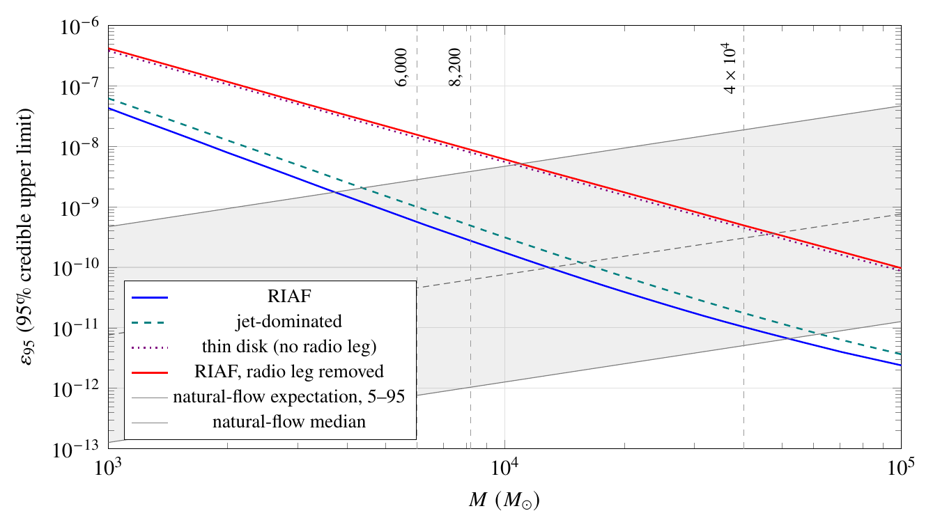
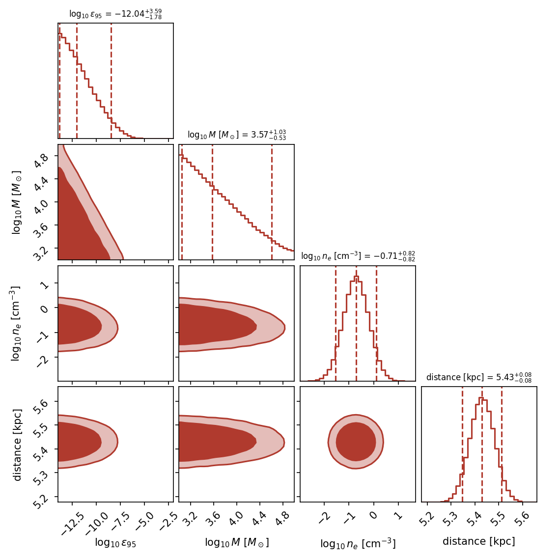
Figure 2 shows the full joint posterior behind these curves over the two parameters of interest and the two dominant nuisances, RIAF family only.
| M (M☉) | RIAF | jet | thin disk | RIAF, no radio | Pexcl (RIAF) | Pexcl (no radio) |
|---|---|---|---|---|---|---|
| 6,000 | 5.7×10⁻¹⁰ | 9.9×10⁻¹⁰ | 1.4×10⁻⁸ | 1.6×10⁻⁸ | 0.19 | 0.004 |
| 8,200 | 2.8×10⁻¹⁰ | 4.9×10⁻¹⁰ | 7.9×10⁻⁹ | 8.8×10⁻⁹ | 0.31 | 0.017 |
| 4×10⁴ | 1.0×10⁻¹¹ | 1.8×10⁻¹¹ | 4.5×10⁻¹⁰ | 5.0×10⁻¹⁰ | 0.90 | 0.44 |
Figure 1 and Table 4 carry the content. Three statements summarize them.
The radio leg dominates wherever the fundamental plane applies. The plane's mass term rises as M0.78 while the Bondi denominator rises as M2, so the radio-driven limit falls as ~M−3.3 and separates from the radio-free curve by 1.5 decades at the top of the mass range. This is the single-object version of the population-level result of Maccarone et al. (2005), Strader et al. (2012), and Tremou et al. (2018): for IMBH masses, radio provides the tightest constraint on quiescent accretion. The plane's extrapolation into deep quiescence is contested (Plotkin et al. 2012), its 0.88-dex scatter is carried as a latent variable rather than a point estimate, and readers who distrust it entirely should quote the red curve: ε95 = 8.8×10⁻⁹ at 8,200 M☉, 5.0×10⁻¹⁰ at 4×10⁴ M☉, from Chandra and JWST with no shared emission model.
Against the natural-flow expectation, the verdict is mass-dependent but no longer only at the top of the range. The grey band is the prediction, εnat = ηADAF(ṁ) fB with ηADAF = 0.1 min(1, ṁhor/10−2)1/2 in Eddington units, following the square-root scaling of the piecewise efficiency fits of Xie & Yuan (2012) as summarized in Yuan & Narayan (2014), evaluated draw-by-draw on the same nuisances. This expectation carries no δFP term, unlike ε95 for the RIAF and jet families, whose radio-leg prediction does (Section 3.3); the fundamental-plane scatter widens the limit but not the band it is compared against, so a reader who distrusts the plane should read the exclusion fractions off the radio-free column rather than treating the asymmetry as a wash. Scoring each natural-flow draw against the measured data directly rather than against a limit marginalized over those same draws, the data reject 85 per cent of that parameter space at the fast-star anchor and 78 per cent at the pulsar-timing point-mass cap under the RIAF family (28 and 20 per cent without the radio leg). At 4×10⁴ M☉ the limit excludes 99 per cent of natural-flow draws, and 76 per cent even using no radio information. Table 6 carries all three figures across the sensitivity ladder. A Bondi-fed hot flow at a 47 Tuc-like density is therefore disfavoured across the contested mass range rather than only at its top: at every anchor something must give, the mass itself, the assumed gas density, or suppression physics beyond the s ≤ 0.5 bracket. The corrected square-root efficiency law is extrapolated three to five decades below the rates it was computed for; holding it flat at the edge of its computed range instead drives every figure above 99 per cent, so this bracket's low end, not its high end, is the conservative reading. This is the paper's principal astrophysical result, and it is invisible in any single-band treatment because it requires the bands and the expectation to share one error budget.
The thin disk is dead everywhere. ε95 for the disk family sits four to five decades below the η ~ 0.06–0.4 a disk radiates at; no Bondi-fed thin disk at any mass in the range survives, quantifying what every prior single-band paper assumed informally.
5.1 The exclusion fraction as a continuous function of mass
Table 4 evaluates Pexcl at three masses because those are the masses the kinematic literature argues about. The Monte Carlo evaluates it on the whole grid, and the continuous version (Figure 3) is the more useful object for a reader who holds a different mass prior than any of the three anchors. It also locates the transitions. Under the RIAF family the exclusion fraction passes 50 per cent at 1.3×10⁴ M☉ and 90 per cent at 4.0×10⁴ M☉; under the jet family the same thresholds fall at 1.6×10⁴ and 4.9×10⁴ M☉. Using no radio information the 50 per cent point moves to 4.8×10⁴ M☉ and the 90 per cent point lies above the grid entirely.
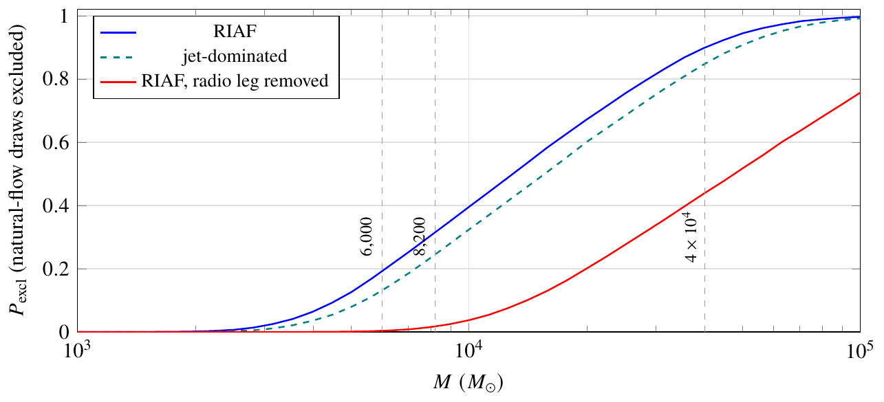
figs/fF_expand_exclcurve.json, which re-exports the grid the v0.3 run already evaluated.5.2 Which band binds which family
Figure 4 shows what the family definitions of Section 3.4 change. At each anchor the figure evaluates the forward model at that family's own ε95 and plots the predicted νLν in every observed band against the published limit in that band, so the three instruments and the three families appear on one axis.
The ordering is family-dependent in the way Section 3.4 claims. For the RIAF family the median predicted radio flux density at ε95 sits at 1.4 times the ATCA 5σ point at 8,200 M☉ and 4.7 times it at 4×10⁴ M☉, while the X-ray prediction sits at 1 per cent of the Chandra bound and the tightest infrared filter at 1 per cent of its own. For the jet family the radio ratios are 1.0 and 3.2 and the F770W ratio rises to 3 per cent, an order of magnitude closer than under the RIAF band fractions and still not competitive with the plane. The thin disk, which carries no radio leg, is bound jointly by F770W (0.28 and 0.38 of the limit) and by the X-ray band (0.26 and 0.36); those two ratios sit within 10 per cent of each other, so for that family the infrared and the X-ray legs share the constraint rather than one dominating.
Ratios above unity for the radio band are expected and are not a detection claim: ε95 is a 95 per cent posterior quantile marginalized over the plane's 0.88-dex latent scatter, so at that εB the median draw predicts a flux the image would have seen while a substantial tail does not. The five-percentile whiskers, which reach two decades below the medians in the radio and a factor of ten in the other bands, are that scatter. And the infrared points are flat across the four filters by construction, since the model predicts one band-peak νLν and each filter constrains it separately; the filters differ only in their limits, which is why F770W sets the infrared constraint.
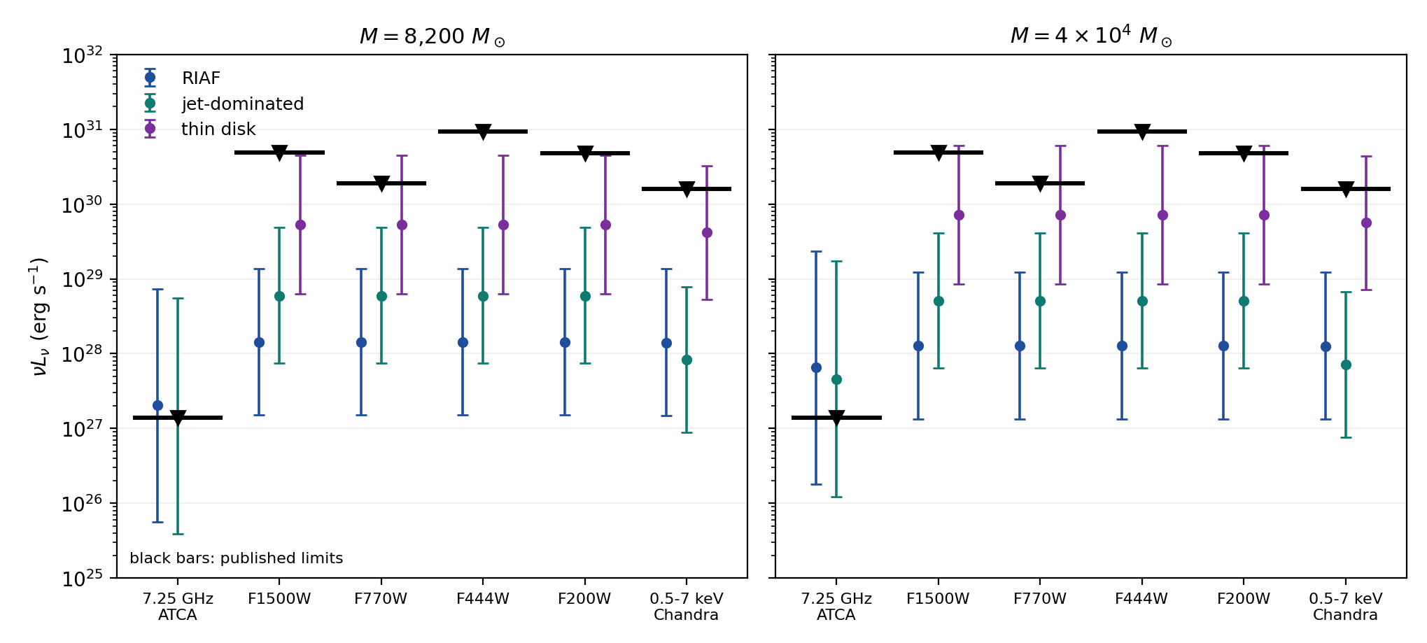
figs/fF_expand_v1.py, numbers in figs/fF_expand_sed.json.5.3 Sensitivity budget
| Variant | 6,000 M☉ | 8,200 M☉ | 4×10⁴ M☉ |
|---|---|---|---|
| baseline | 5.7×10⁻¹⁰ | 2.8×10⁻¹⁰ | 1.0×10⁻¹¹ |
| ne prior widened to 1.5 dex | 3.2×10⁻⁹ | 1.6×10⁻⁹ | 7.3×10⁻¹¹ |
| ne prior median ÷ 10 | 3.5×10⁻⁹ | 1.6×10⁻⁹ | 4.3×10⁻¹¹ |
| widened + wind floor (ne ≥ 0.05) | 6.4×10⁻¹⁰ | 3.2×10⁻¹⁰ | 1.2×10⁻¹¹ |
| εB-grid floor raised to 10−11 | 4.6×10⁻⁹ | 2.8×10⁻⁹ | 3.6×10⁻¹⁰ |
| Variant | RIAF | RIAF, no radio | ||||
|---|---|---|---|---|---|---|
| 6,000 | 8,200 | 4×10⁴ | 6,000 | 8,200 | 4×10⁴ | |
| baseline | 0.19 | 0.31 | 0.90 | 0.00 | 0.02 | 0.44 |
| ne prior widened to 1.5 dex | 0.16 | 0.22 | 0.63 | 0.03 | 0.05 | 0.26 |
| ne prior median ÷ 10 | 0.00 | 0.01 | 0.46 | 0.00 | 0.00 | 0.02 |
| widened + wind floor (ne ≥ 0.05) | 0.26 | 0.38 | 0.87 | 0.07 | 0.11 | 0.48 |
| εB-grid floor raised to 10−11 | 0.03 | 0.07 | 0.48 | 0.00 | 0.00 | 0.32 |
| X-ray limit read two-sided 95 per cent | 0.19 | 0.32 | 0.90 | 0.00 | 0.02 | 0.45 |
| X-ray limit read as 3σ | 0.20 | 0.32 | 0.90 | 0.01 | 0.03 | 0.47 |
| IR completeness row 99.7 per cent | 0.19 | 0.31 | 0.90 | 0.00 | 0.01 | 0.42 |
| IR completeness row 68 per cent | 0.20 | 0.32 | 0.90 | 0.01 | 0.02 | 0.46 |
| IR tightest single filter only | 0.19 | 0.31 | 0.90 | 0.00 | 0.02 | 0.43 |
| Bondi denominator, Paper E convention | 0.12 | 0.24 | 0.84 | 0.00 | 0.01 | 0.35 |
Table 6 prices the headline verdict rather than the limit behind it, and the two do not move together. Widening the ne prior relaxes ε95 by a factor 7 at the high anchor but costs the exclusion fraction only 0.27, because a log-normal's median is unchanged by a width change: what widens is the expectation band, not its centre. Shifting the prior centre is the case with no cancellation, since ε95 loosens by a factor 4 while the natural-flow median falls by a factor 10, and the two effects compound; that row alone sets the lower end of the range. The wind-replenishment floor works the other way, raising the natural-flow median by 1.8 while leaving ε95 near baseline, so the astrophysically defended envelope strengthens the verdict at the two lower anchors. Across every convention choice in this paper the exclusion fraction at 4×10⁴ M☉ stays at 0.90, and across the density variants it is bounded below by 0.46. The radio-free column is the fragile one, spanning 0.02 to 0.48, and the 44 per cent figure should be read with that range attached.
Table 5 is the quantified version of Section 3.2's caveat. Widening the ne prior by a decade in each direction, or dividing its median by ten, each relax ε95 by a factor ~6: the curve's normalization belongs to the gas-density assumption, in both its width and its center, and no claim in this paper escapes that conditioning. Two things bound the damage. The wind-replenishment floor of Section 4 truncates the low-density tail on astrophysical grounds, and with it in place the widened prior returns almost to baseline. And the εB-prior floor matters as it always does for non-detections, a factor ~10 when the grid floor rises three decades; every ε95 in this paper is quoted on the 10−14 grid, and the machine-readable likelihood tables let any reader impose their own.
5.3.1 Which nuisance carries the spread
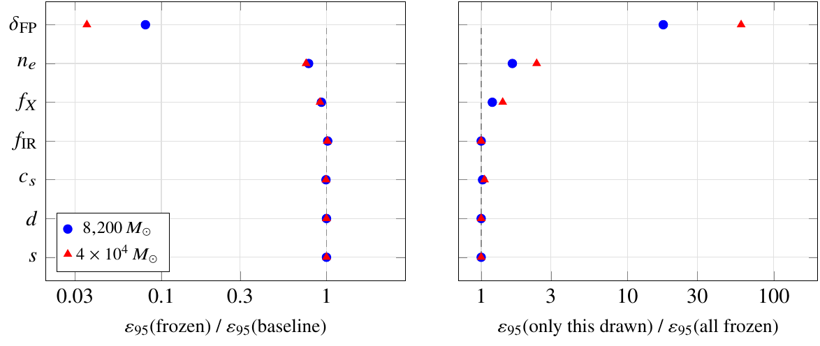
Table 5 varies analysis choices. The seven nuisance parameters can be interrogated separately, by re-running the same posterior with one of them held at its prior's central value while the other six are drawn, and again with only that one drawn and the other six held (Figure 5). The two views answer different questions: the first asks how much of the limit's looseness a given parameter is responsible for, the second asks how much looseness that parameter would produce on its own.
The answer is that the fundamental plane's latent scatter carries the spread. Freezing δFP at zero tightens ε95 by a factor of 12.5 (~13) at 8,200 M☉ and ~28 at 4×10⁴ M☉; drawing it alone, with everything else fixed, reproduces a limit 18 and 60 times looser than the fully frozen case. No other parameter comes within an order of magnitude. The gas density is second and is a distant second in this accounting: freezing it tightens ε95 by 22 to 25 per cent, and drawing it alone loosens the frozen limit by a factor 1.6 to 2.4. The X-ray band fraction contributes 6 to 9 per cent, the sound speed under 1 per cent, and the distance nothing measurable, as expected from a 1 per cent prior. The infrared band fraction moves the RIAF limit by 2 per cent in the opposite direction, which is the signature of a leg that never binds in this family.
The distance prior and the suppression index are inert here, for structural reasons worth naming. The distance prior is narrow enough that its 1 per cent width cannot register against the plane's 0.88 dex. The suppression index s does not enter the likelihood at all: it sets the natural-flow expectation εnat against which the limit is compared, not the limit itself, so its entire influence in this paper runs through Pexcl and the grey band of Figure 1 rather than through ε95.
This does not contradict Section 3.2's statement that the gas density owns the result. The two statements are about different things. Within the stated priors, the plane's scatter is what widens the posterior; the density's danger is in the choice of prior centre, which no freezing test can expose, and which Table 5's prior-shift rows price at a factor ~6. A reader who distrusts the plane has the radio-free curve; a reader who distrusts the density analogy has the shift rows and the wind floor.
figs/fF_expand_nuisance.json.5.4 Where this sits against the survey population
The single-cluster depth used here is best read against the 50-cluster MAVERIC survey (Tremou et al. 2018), which is the reference population for radio IMBH limits and the source of the field's null (Table 7). Two cautions travel with the comparison. First, each entry assumes its own distance: Tremou et al. (2018) adopt 4.9 kpc for ω Cen, Haggard et al. (2013) 5.2 kpc, Chen et al. (2025) and Mahida et al. (2026) 5.49 kpc, against this paper's 5.43 kpc prior. The spread is ordinary paper-to-paper variation and it propagates as d2 into any luminosity, so the flux densities compare directly while the derived quantities do not. Second, the survey's mass limits are obtained by inverting the fundamental plane, the step Section 3.3 declines to take; they are quoted here as the literature's own currency and are not εB and not convertible to it without the full nuisance treatment.
| Dataset | Depth | Derived limit | Assumed d |
|---|---|---|---|
| MAVERIC ATCA, ω Cen (Tremou et al. 2018) | <8.8 μJy (3σ) | M < 1000 M☉ | 4.9 kpc |
| MAVERIC VLA stack, 24 clusters | 0.65 μJy beam−1 | M < 800 M☉ | per cluster |
| MAVERIC ATCA stack, 14 clusters | 1.42 μJy beam−1 | M < 970 M☉ | per cluster |
| This paper's radio input (Mahida et al. 2026) | 1.1 μJy beam−1 rms | see Figure 1 | 5.49 kpc |
The ATCA campaign of Mahida et al. (2026) is deeper on one cluster than the MAVERIC stack is on 24, which is what makes a per-object posterior worth building at all. Three ambiguities in the survey paper are carried rather than resolved: its ω Cen flux limit appears as 8.8 μJy in Table 2 and 8.9 μJy in Section V.2.1; its VLA stack mass limit is given as both <800 and <730 M☉ in a single sentence, and we quote the weaker; and whether ω Cen enters the 14-cluster ATCA stack is not stated, though the paper's explicit exclusion list omits it. Its comparison of the ω Cen radio limit against Haggard et al. (2013) also cites the X-ray limit as 1.7×1030 erg s−1 where Haggard et al. state 1.6×1030, which looks like a transcription rounding. None of this affects the numbers of Section 5, which use no MAVERIC input; it affects only what the reader should do with the row above.
6. The duty-cycle loophole
The three inputs sample time very differently, and Mahida et al. (2026)'s Table 1 makes the radio sampling explicit: 25 observing blocks across three ATCA projects, 2010 January 22 to 2024 December 27, summing to 177.19 hr on source (CX556, 20 blocks, 147.09 hr; C2877, 3 blocks, 11.79 hr; C2158, 2 blocks, 18.31 hr). Those rows exceed the ~170 hr of the paper's abstract and the 172 hr of its Section II.3; we report the sum as printed and leave the reconciliation to that paper, noting that prose totals quoted after flagging would run below a raw table sum rather than above it. Chandra contributes four exposures in two epochs twelve years apart, JWST a single epoch.
Two consequences follow on different timescales. For variability slower than the sampled span, the limits above apply to the time-average δ εon of a flow active a fraction δ of the time at εon, so εon ≲ ε95/δ; the radio image is a weighted combination over the full fourteen-year span, so this is the operative statement there. For variability faster than a block, the source must be off during every epoch to escape, which for N ≃ 30 independent epochs (25 radio blocks, four Chandra exposures, one JWST visit) gives a miss probability (1−δ)N reaching 50 per cent only near δ ≈ 0.02. This order-of-magnitude estimate counts every block or exposure as one independent trial regardless of its duration relative to the assumed flare timescale τ; Section 6.1's block-by-block treatment does not carry that assumption and supersedes this estimate in rigor. The excluded region is therefore the band εon > ε95/δ down to a few per cent duty cycle, and effectively nothing below that: a flow that spends 99 per cent of its time off is constrained only by the luck of the sampling. An earlier draft put the epoch count at N ~ 6 and the sampling break at δ ≈ 0.1, having treated the radio campaign as one epoch. This is the standard loophole of every quiescent-limit paper, here made explicit because Paper E's tidal-disruption arithmetic predicts exactly such intermittency on 107-yr recurrence with 10−4 duty, far below the reach of any current sampling; nothing in this paper's nulls bears on that channel, in either direction.
6.1 What the block list actually excludes
The block list supports a stronger statement than a miss probability, because each block is an image in its own right. Scaling the combined image's sensitivity by on-source time, σi = 1.1 μJy √(177.19 hr / ti), the 25 blocks reach 4.5 to 12.0 μJy rms with a median of 5.3 μJy over a median 7.6 hr on source, so a single block detects a source at 5σ near 27 μJy while the combined image reaches 5.5 μJy. That scaling assumes each on-source hour is equally sensitive across the three projects and both observing frequencies, which Mahida et al. (2026) do not state block by block; it is the only scaling their published table supports.
A flare train is then a two-parameter object: amplitude S and duration τ, recurring with period Trec at an unknown phase. Laying such a train over the real block timeline (2010 January 22 to 2024 December 27, a 14.9-yr span containing 177.19 hr of on-source time) and asking whether any single block's τ-averaged flux exceeds its own 5σ point, or the campaign mean exceeds 5.5 μJy, gives a detection probability over phase. Table 8 reports, for each (S, τ), the longest recurrence interval that would still have been caught in at least 95 per cent of phases. Anything recurring faster than that is excluded; anything slower is not.
| Flare amplitude | τ = 0.5 hr | 2 hr | 8 hr | 24 hr |
|---|---|---|---|---|
| 10 μJy | – | – | 12 (0.655) | 31 (0.763) |
| 30 μJy | – | 8 (0.263) | 25 (0.322) | 130 (0.184) |
| 100 μJy | 8 (0.066) | 31 (0.064) | 130 (0.061) | 209 (0.115) |
| 300 μJy | 15 (0.032) | 81 (0.025) | 130 (0.061) | 209 (0.115) |
| 1 mJy | 81 (0.006) | 81 (0.025) | 130 (0.061) | 209 (0.115) |
Low-amplitude trains are excluded only when they are almost always on: a 10 μJy source is invisible in any single block and can be caught only through the campaign mean, which requires a duty cycle above 0.7. Bright, brief trains are bounded by the sampling rather than by the sensitivity: at 300 μJy and above, for durations of 2 hr and longer, the exclusion saturates near a recurrence interval of 3 to 9 days, because 177 hr of on-source time spread over 14.9 yr covers 0.14 per cent of the span, and a flare that recurs more slowly than about a week simply misses every block most of the time no matter how bright it is. Between those regimes the campaign excludes real parameter space: a 100 μJy, 2-hr flare is excluded for recurrence faster than 31 hr, a duty cycle of 6×10⁻².
The scaling's own uncertainty can be priced. Drawing per-block sensitivity log-normally about it, at fixed combined campaign sensitivity, since the 1.1 μJy combined rms is measured rather than assumed, moves the table where the single-block channel sets the threshold and leaves it alone where the campaign mean does. At 0.2 dex of scatter, two of the fourteen well-determined cells move by one grid step: the 30 μJy, 24-hr threshold falls from 130 to 81 hr and the 100 μJy, 2-hr threshold from 31 to 25 hr. Both 10 μJy rows hold to the digit at every scatter level tested, up to 0.3 dex, because a 10 μJy source is caught only through the campaign mean, whose depth is measured. The floor of the excluded region is likewise unaffected at ±30 per cent per-block rms, and reaches a duty cycle of 1×10⁻² only at 0.3 dex. The caveat this paragraph opens with therefore attaches to the mid-amplitude, long-duration cells rather than to the faint end, which the source paper's combined image already constrains directly. Numbers in figs/fF_calcF1_duty_band.json.
The floor of the excluded region is therefore a duty cycle of 6×10⁻³, reached at 1 mJy and half an hour, and it is set by sampling coverage rather than by image depth. This tightens the order-of-magnitude estimate above by a factor of a few and it changes the instrument implication: for the flare channel, more epochs at the present depth would buy more than the same time added to a single deep image, which is the opposite of the priority ordering that Section 7 gives for the steady channel. Paper E's predicted tidal-disruption intermittency, at 10−4 duty on 107-yr recurrence, remains two decades below the floor and 12 decades outside the recurrence range, so the conclusion of the preceding paragraph is unchanged: this campaign says nothing about that channel.
7. Forecasts
Three measurements would harden or move the curves, in descending order of leverage per unit effort.
A measured core density. The 19-pulsar timing set (Colom i Bernadich et al. 2026) makes an ω Cen dispersion-measure gas detection feasible for the first time, by the method that measured 47 Tuc (Freire et al. 2001; Abbate et al. 2018); the caveat, that DM gradients constrain the column through the pulsar volume rather than the density at the hole, is real and enters as geometry. The forecast gain on ε95 itself is modest (a ±10 per cent density measurement tightens the baseline by ~22 per cent, since the 0.5-dex prior is already informative). A measurement converts every curve from analogy-conditional to measured, removes the largest single objection to the enterprise, and, if the density comes in low, legitimately weakens the bounds when the conditions are tested.
Table 9 is the requirement that forecast implies, computed from the published timing set. All 19 pulsars have measured dispersion measures; eight have them from full timing solutions with formal uncertainties of 5×10⁻⁵ to 1.3×10⁻³ pc cm−3, and five of those eight also have a measured first DM derivative. Timing precision is not the obstacle.
Geometry sets what a dispersion-measure gradient can reach. Gas filling the cluster core, a uniform sphere of the catalogue core radius 2.37′ (Harris 1996), or 3.74 pc at 5.43 kpc, imprints a central-chord excess of 0.75 pc cm−3 at ne = 0.1 cm−3, and 13 of the 19 sight lines pass inside it. Gas confined to the influence radius of the hole, the 0.4 pc region the Bondi rate is actually about, imprints 0.08 pc cm−3 and no published sight line passes through it: the innermost pulsar, H at 0.56′, projects to 0.88 pc. A DM determination therefore measures the core-filling component and reaches the Bondi-scale density only through an assumed profile, which is the caveat named above, now with a number attached.
The sight-line scatter sets how well it can be measured. The 19 published DMs span 94.3 to 102.6 pc cm−3 with an r.m.s. of 2.9 pc cm−3, three orders of magnitude above the per-pulsar measurement precision and four times the signal a core-filling ne = 0.1 cm−3 would produce. Fitting the chord template plus a free foreground constant to the 19 measurements by least squares returns an amplitude of −0.33 ± 0.24 cm−3, consistent with zero and formally negative, with a residual r.m.s. of 2.8 pc cm−3. We do not quote the implied upper limit as a constraint on the cluster's gas: a model whose residuals exceed its measurement errors by three orders of magnitude is falsified by its own fit, and the formal error bar of a falsified model is not a credible interval. What the fit does establish is the requirement. At the present per-sight-line scatter, a 3σ determination of ne = 0.1 cm−3 needs the scatter modelled down by a factor of 7, or of order 103 sight lines at the current scatter, which no foreseeable timing programme will deliver. The tractable path is the former: the excess scatter is structure, in the Galactic foreground or in the cluster, and it is measurable in its own right through the DM derivatives that five of these pulsars already have.
| PSR J1326−4728 | θ (′) | b (pc) | DM (pc cm−3) | σDM | ΔDM at 0.1 cm−3 |
|---|---|---|---|---|---|
| H | 0.56 | 0.88 | 98.1716 | 0.0005 | 0.73 |
| B | 0.76 | 1.20 | 100.2806 | 0.0008 | 0.71 |
| F | 1.00 | 1.58 | 98.29 | – | 0.68 |
| P | 1.00 | 1.58 | 102.17 | – | 0.68 |
| O | 1.50 | 2.37 | 94.305 | – | 0.58 |
| E | 1.58 | 2.50 | 94.33967 | 5×10⁻⁵ | 0.56 |
| J | 1.80 | 2.84 | 97.28 | – | 0.49 |
| K | 1.89 | 2.99 | 94.7836 | 0.0007 | 0.45 |
| A | 1.93 | 3.05 | 100.3267 | 0.0004 | 0.43 |
| G | 1.96 | 3.10 | 99.7445 | 0.001 | 0.42 |
| C | 1.98 | 3.13 | 100.6643 | 0.0013 | 0.41 |
| Q | 2.30 | 3.63 | 95.923 | – | 0.18 |
| S | 2.32 | 3.66 | 96.24 | – | 0.15 |
| M | 2.40 | 3.79 | 101.47 | – | 0 |
| D | 2.50 | 3.95 | 96.5462 | 0.0009 | 0 |
| N | 2.66 | 4.20 | 102.1 | – | 0 |
| L | 3.32 | 5.24 | 101.4759 | – | 0 |
| I | 3.53 | 5.58 | 102.555 | – | 0 |
| R | 3.90 | 6.16 | 102.2 | – | 0 |
Deeper radio. The radio-leg limit scales as σS1/0.60. A tenfold rms improvement (SKA-Mid-era depth, ~0.1 μJy) tightens the RIAF ε95 by an order of magnitude at every anchor (2.8×10⁻¹⁰ → 2.5×10⁻¹¹ at 8,200 M☉), pushing the natural-flow exclusion fraction at the fast-star anchor from 31 to 62 per cent, and from 90 to 99 per cent at 4×10⁴ M☉.
Deeper mid-infrared. Under the RIAF family, deeper MIRI photometry changes nothing (the X-ray leg dominates it in every draw; JWST's role there is the independent-systematics cross-check). Under the jet-dominated family it is the binding band, and with the per-filter treatment of Section 2 a threefold depth gain moves ε95 by 29 per cent at the fast-star anchor (31 per cent at 6,000 M☉, 21 per cent at 4×10⁴ M☉). That is a real gain, an order of magnitude short of what the same effort buys in the radio, and it is larger than the ~7 per cent an earlier draft reported under the single-constant infrared proxy. The instrument-priority implication for Paper C is stated in those terms: radio first, density second, mid-infrared as discrimination between families rather than depth.
8. Scope of the adjudication
Under the null reading, the center is gas-starved or its flow is suppressed: at the pulsar-timing and fast-star anchors, Figure 1 leaves natural-flow parameter space comfortably open, and nothing forces an exotic conclusion. At the high-mass anchor the null reading now pays a price: it must give up one of its own ingredients, the mass, the fiducial density, or the standard suppression bracket. That is a constraint on conventional astrophysics, publishable and testable on its own terms, and it sharpens the mass tension from the accretion side: the same high-mass range favored by the fast-star kinematics is the range where electromagnetic silence is hardest to buy naturally. Under the engineered reading of Papers A and E, a system extracting accretion power as work rather than radiation presents a deep multi-band null as its expected signature, at any mass; the data cannot separate that reading from the null, and this paper does not claim otherwise. What it contributes to that adjudication is the currency: a likelihood over εB with stated conditioning, which Paper E's framework ingests in place of the single-band, single-convention numbers it previously had to translate. The duty-cycle loophole of Section 6 is charged to both readings equally.
9. Conclusion
The deepest radio, infrared, and X-ray observations of ω Cen's center jointly admit a posterior on the Bondi radiative efficiency of any central accretion flow: ε95 = 2.8×10⁻¹⁰ at the fast-star mass anchor for a RIAF-like flow under the stated priors, 8.8×10⁻⁹ with no radio information, and an order of magnitude tighter at the top of the contested mass range, where the limits now exclude 90 per cent of the parameter space of a natural suppressed hot flow at the fiducial gas density, and above 46 per cent across the density priors of Table 7. The curve's normalization is owned by the unmeasured central density; the cluster's own stellar winds bound that density from below, the current pulsar set can measure it, and until it does, Figure 1 is the quantitative meaning of ω Cen's silence. The single observation that converts these limits from analogy-conditional to measured is a DM-gradient fit to the 19-pulsar set at the ±10 per cent level (§8.1). Both the gas-starvation null at moderate masses and the engineered-silence hypothesis of this paper set live inside it; a high-mass IMBH feeding naturally at the fiducial density no longer does.
Data availability
The posterior script (figs/fF_posterior_v3.py, fixed seed), its full output (figs/fF_v3_results.json), the exclusion-fraction tables, the measured-input provenance file that supplies every observational number used above with its source location and verbatim quotation (figs/fF_measured_inputs.json) together with the derived epoch and survey-context exports (figs/fF_epochs.json, figs/fF_maveric_context.json), the superseded v0.2 script and output retained for comparison, the appendix cross-check script (figs/fF_joint_bound.py) and its output (figs/fF_results.json), the expansion-analysis script behind Figures 2, 3 and 4 and Tables 8 and 9 (figs/fF_expand_v1.py, fixed seed, with its outputs fF_expand_nuisance.json, fF_expand_sed.json, fF_expand_exclcurve.json, fF_expand_duty.json and fF_expand_dm.json), and the figure coordinate tables are distributed with the paper source at omegacentauri.me. The pulsar dispersion measures of Table 10 are read from the timing-set extraction h/data/pulsars.json, which records each value's source location in Colom i Bernadich et al. (2026). The provenance file also records two internal inconsistencies in the sources that a reader checking our inputs will meet: Mahida et al. (2026)'s conservative efficiency limit is stated as 4×10⁻³ in their abstract and Section IV.1 and as 4×10⁻⁶ in their Section V, and their Table 1 observing hours exceed their own prose totals. Neither enters any number in this paper, and both are flagged here for that paper's authors.
The analysis would improve with, and the machinery directly ingests, the measured central-pixel flux density and its uncertainty from the ATCA image, the per-epoch Chandra source counts and background at the center list, and the per-filter MIRI/NIRCam limiting fluxes; we request them from the respective teams.
Appendix A. Conventions, unit conversions, and cross-paper reconciliation
Bondi rate. Equation 1 uses the γ = 5/3 eigenvalue λ = 0.25 and a gas-rest-frame denominator cs3, with cs drawn between the μ = 0.6 isothermal value (11.7 km s−1) and the pure-hydrogen adiabatic value (16.6 km s−1) at 104 K. Paper E's fuel budget (its Eq. 2) uses λ = 1 with a (σ2+cs2)3/2 denominator as a turbulent-medium convention; the net ratio between the two conventions is 0.25 (σ2+cs2)3/2/cs3 ≃ 1.9 at the fiducial values, i.e. this paper's ṀB is ≃ 1.9× Paper E's at equal (M, ne), and its εB limits are correspondingly ≃ 1.9× tighter than they would be under E's convention. At 2×10⁴ M☉ and median nuisances, Equation 1 gives ṀB = 5.3×10¹⁸ g s−1 against E's 3×10¹⁸; both statements are correct within their stated conventions.
Electron mean molecular weight. μe = 2/(1+X) = 1.17 at X = 0.71. An earlier draft used 1.5, which corresponds to no physical composition and tightened all limits by 27 per cent; corrected here.
Radio. LR ≡ νLν at 5 GHz under a flat spectrum: LR = 4πd2 (5 GHz) Sν, with Sν the 7.25 GHz flux density (Lν flat). At d = 5.43 kpc, 1.1 μJy corresponds to LR = 1.9×1026 erg s−1 (5.8×1026 at 3σ).
X-ray bands. The fundamental plane is calibrated on 2–10 keV; the Chandra limit is 0.5–7 keV; F(2–10)/F(0.5–7) = ln(10/2)/ln(7/0.5) = 0.61 for Γ = 2.
X-ray reference distance. Haggard et al. (2013) adopt 5.2 kpc (their abstract and Table 1, from the Harris catalogue). An earlier draft of this paper carried 4.8 kpc for that reference and warned that the mismatch against the 5.43 kpc prior shifts the X-ray leg by 28 per cent. Both halves of that warning were wrong. The distance is 5.2 kpc, and the shift is zero regardless: the X-ray likelihood is evaluated on flux, which is what Chandra measured and is distance-independent, so the drawn distance enters the predicted flux and never the limit. The reference distance now serves as a consistency check on the source's own numbers: 4πD2 fX,lim = 1.62×1030 erg s−1 at 5.2 kpc against the 1.6×1030 Haggard et al. (2013) state, which holds at their distance and fails at 4.8 kpc (1.38×1030). The script asserts it at run time. The infrared limits, by contrast, are published as luminosities and do carry their source distance, so they are referenced at Chen et al.'s 5.49 kpc and rescaled draw by draw.
Run-time self-checks. Two consistency assertions accompany the shipped code and print their result rather than assuming it, the discipline of Paper H's self-audit: the expansion script (figs/fF_expand_v1.py) reproduces the RIAF anchors of Table 4 against fF_v3_results.json and asserts the match at run time before proceeding; the Haggard luminosity-anchor check above asserts 4πD2fX,lim against Haggard et al.'s stated 1.6×1030 erg s−1 at their own distance. Both assertions halt the build on failure, so a compiled paper carries their pass by construction; neither prints a numeric residual beyond the values already quoted above.
Confidence conventions. Each leg uses the confidence its source states, mapped through the normal quantile. The X-ray limit is one-sided 95 per cent (z = 1.645); the infrared limits are taken at the 95 per cent completeness row on the same convention. Neither choice is load-bearing:
| Leg | Convention | 6,000 M☉ | 8,200 M☉ | 4×10⁴ M☉ |
|---|---|---|---|---|
| X-ray | one-sided 95 % (z = 1.645, primary) | 5.68×10⁻¹⁰ | 2.75×10⁻¹⁰ | 1.03×10⁻¹¹ |
| X-ray | two-sided 95 % (z = 1.960) | 5.62×10⁻¹⁰ | 2.73×10⁻¹⁰ | 1.03×10⁻¹¹ |
| X-ray | earlier draft's lim/3 | 5.42×10⁻¹⁰ | 2.64×10⁻¹⁰ | 1.01×10⁻¹¹ |
| IR | 99.7 % completeness row | 5.86×10⁻¹⁰ | 2.83×10⁻¹⁰ | 1.05×10⁻¹¹ |
| IR | 95 % completeness row (primary) | 5.68×10⁻¹⁰ | 2.75×10⁻¹⁰ | 1.03×10⁻¹¹ |
| IR | 68 % completeness row | 5.45×10⁻¹⁰ | 2.65×10⁻¹⁰ | 1.01×10⁻¹¹ |
| IR | tightest single filter, 95 % | 5.76×10⁻¹⁰ | 2.79×10⁻¹⁰ | 1.04×10⁻¹¹ |
The X-ray ladder spans 5 per cent on these anchors and the infrared ladder 8 per cent. On the jet family, where the infrared leg binds, the tightest-single-filter reading gives 1.04×10⁻⁹, 5.07×10⁻¹⁰ and 1.80×10⁻¹¹ against the combination's 9.93×10⁻¹⁰, 4.89×10⁻¹⁰ and 1.76×10⁻¹¹, a 5 per cent effect, because F770W dominates the combination in any case. Holding the infrared limits at this paper's 5.43 kpc instead of Chen et al.'s 5.49 kpc moves the jet anchors by 0.5 per cent.
Reconstruction of the limit legs. A published bound states P(observed < flim), which is a survival statement, while Section 3.3 evaluates a Gaussian centred at zero with the same σ. Substituting the survival form on the X-ray and infrared legs, the two published as limits with no central value, moves the RIAF and jet anchors by 1 per cent or less and leaves every exclusion fraction unchanged to three decimals; on the radio-free curve, where those legs are the only legs, it loosens the anchors by 29 to 30 per cent (X-ray alone 13 to 15, infrared alone 10 to 12). The radio leg is excluded from this substitution because Mahida et al. (2026) report a measured central flux density rather than a bound, and a survival form there would discard the measurement; doing so anyway loosens the RIAF anchors by a factor 3 to 4, which is the value of the measurement rather than a property of the reconstruction. An injection study of 200 realizations per cell puts the coverage of the 95 per cent upper limit at 0.91 at 8,200 M☉ and 0.96 at 4×10⁴ M☉ when the true εB sits at the published limit, against a binomial uncertainty of 0.015, so the convention is calibrated to a few percentage points and slightly under-covers at the lower anchor. Numbers in figs/fF_calcF1_hybrid.json and figs/fF_calcF1_coverage.json.
Cross-paper exchange rates. At the common reference point (M = 2×10⁴ M☉, ne = 0.23 cm−3, median nuisances): this paper's εB relates to the horizon-side efficiency as η = εB/fB with fB ∈ [10−4.1, 10−2.5]; Mahida et al. (2026)'s bounded quantity is an accretion fraction under their assumed radiative model and is neither εB nor η; Haggard et al. (2013)'s 10−6–10−8 is an εB-like quantity under their fixed density and mass and maps to εB ≈ (0.5–1.5)× their value once the density and λ conventions are aligned. Exact re-evaluation of both published numbers in this paper's convention requires parameters stated only in their full texts and is deferred to the journal version; until then the qualitative ordering (radio strongest, X-ray next, IR family-dependent) is convention-independent.
Appendix B. Threshold-inversion cross-check
An earlier construction of this bound (script figs/fF_joint_bound.py, retained unchanged with its own seed and output) inverted the per-band thresholds as that draft labelled them, 3σ in every band, through the same nuisance draws and reported percentiles of the per-draw minimum. It is transparent and reproducible, and its 95th-percentile "conservative" values (1.5×10⁻⁸ at 8,200 M☉ with the radio leg; 3.0×10⁻⁷ without) sit one to two decades above the credible limits of Table 4, for two reasons with opposite signs: the threshold construction discards the information in the measured values (weakening), and its percentile is a nuisance-prior quantile of a limit rather than a posterior statement about εB (not comparable in coverage). The disagreement is largest where the fundamental-plane tail dominates, as expected. Its X-ray threshold also predates the confidence relabelling of Section 2, which is a further reason the two constructions are not expected to agree numerically. The posterior supersedes it; it remains in the distribution as a check that no single modeling choice in Section 3.3 drives the headline numbers by itself.
References
- Abbate, F., Possenti, A., Ridolfi, A., Freire, P. C. C., Camilo, F., Manchester, R. N., and D'Amico, N. (2018). Internal gas models and central black hole in 47 Tucanae using millisecond pulsars. Monthly Notices of the Royal Astronomical Society, 481(1):627–637. doi:10.1093/mnras/sty2298
- Bañares-Hernández, A., Calore, F., Martín Camalich, J., and Read, J. I. (2025). New constraints on the central mass contents of Omega Centauri from combined stellar kinematics and pulsar timing. Astronomy & Astrophysics, 693:A104. arXiv:2408.00939 · doi:10.1051/0004-6361/202451763
- Blandford, R. D. and Begelman, M. C. (1999). On the fate of gas accreting at a low rate on to a black hole. Monthly Notices of the Royal Astronomical Society, 303:L1–L5. doi:10.1046/j.1365-8711.1999.02358.x
- Chatterjee, P., Hernquist, L., and Loeb, A. (2002). Dynamics of a massive black hole at the center of a dense stellar system. The Astrophysical Journal, 572:371–381. doi:10.1086/340224
- Chen, S., Hare, J., Kargaltsev, O., Yang, H., Cioffi, D., Häberle, M., and Seth, A. (2025). The intermediate mass black hole in Omega Centauri: Constraints on accretion from JWST. Submitted to ApJ. arXiv:2511.20945
- Colom i Bernadich, M., Dai, S., Abbate, F., Kerr, M., Bachetti, M., Buchner, S., Johnston, S., Burgay, M., Possenti, A., Ridolfi, A., Freire, P. C. C., Kramer, M., Stappers, B., et al. (2026). A joint MeerKAT and Parkes view of Omega Centauri: New TRAPUM searches and pulsar timing. arXiv e-prints, page arXiv:2603.21845. Under review. arXiv:2603.21845
- Di Cintio, P., Pasquato, M., Barbieri, L., Trani, A. A., and Di Carlo, U. N. (2023). Dynamics of intermediate mass black holes in globular clusters. Wander radius and anisotropy profiles. Astronomy & Astrophysics, 673:A8. arXiv:2302.05542 · doi:10.1051/0004-6361/202346124
- Freire, P. C., Kramer, M., Lyne, A. G., Camilo, F., Manchester, R. N., and D'Amico, N. (2001). Detection of ionized gas in the globular cluster 47 Tucanae. The Astrophysical Journal Letters, 557:L105–L108. doi:10.1086/323248
- Häberle, M., Neumayer, N., Seth, A., Bellini, A., Libralato, M., Anderson, J., Whitaker, M., van de Ven, G., Watkins, L. L., Clontz, C., et al. (2024). Fast-moving stars around an intermediate-mass black hole in ω Centauri. Nature, 631(8020):285–289. arXiv:2405.06015 · doi:10.1038/s41586-024-07511-z
- Haggard, D., Cool, A. M., Heinke, C. O., van der Marel, R., Cohn, H. N., Lugger, P. M., and Anderson, J. (2013). A deep Chandra X-ray limit on the putative IMBH in Omega Centauri. The Astrophysical Journal Letters, 773:L31. arXiv:1307.6217 · doi:10.1088/2041-8205/773/2/L31
- Harris, W. E. (1996). A catalog of parameters for globular clusters in the Milky Way. The Astronomical Journal, 112:1487. doi:10.1086/118116
- Lu, T.-N. and Kong, A. K. H. (2011). Radio continuum observations of 47 Tucanae and ω Centauri: Hints for intermediate-mass black holes? The Astrophysical Journal Letters, 729:L25. arXiv:1102.1668 · doi:10.1088/2041-8205/729/2/L25
- Maccarone, T. J., Fender, R. P., and Tzioumis, A. K. (2005). Upper limits on central black hole masses of globular clusters from radio emission and a possible black hole detection in the Ursa Minor dwarf galaxy. Monthly Notices of the Royal Astronomical Society, 356:L17–L22. doi:10.1111/j.1745-3933.2004.08584.x
- Mahida, A. D. et al. (2026). No evidence for accretion around the intermediate-mass black hole in Omega Centauri. The Astrophysical Journal, 996:122. arXiv:2512.09649 · doi:10.3847/1538-4357/ae2ad4
- Merloni, A., Heinz, S., and Di Matteo, T. (2003). A fundamental plane of black hole activity. Monthly Notices of the Royal Astronomical Society, 345:1057–1076. doi:10.1046/j.1365-2966.2003.07017.x
- Noyola, E., Gebhardt, K., and Bergmann, M. (2008). Gemini and Hubble Space Telescope evidence for an intermediate-mass black hole in ω Centauri. The Astrophysical Journal, 676:1008–1015. arXiv:0801.2782 · doi:10.1086/529002
- Noyola, E., Gebhardt, K., Kissler-Patig, M., Lützgendorf, N., Jalali, B., de Zeeuw, P. T., and Baumgardt, H. (2010). Very large telescope kinematics for omega Centauri: Further support for a central black hole. The Astrophysical Journal Letters, 719:L60–L64. arXiv:1007.4559 · doi:10.1088/2041-8205/719/1/L60
- Plotkin, R. M., Markoff, S., Kelly, B. C., Körding, E., and Anderson, S. F. (2012). Using the fundamental plane of black hole activity to distinguish X-ray processes from weakly accreting black holes. Monthly Notices of the Royal Astronomical Society, 419:267–286. arXiv:1105.3211 · doi:10.1111/j.1365-2966.2011.19689.x
- Strader, J., Chomiuk, L., Maccarone, T. J., Miller-Jones, J. C. A., Seth, A. C., Heinke, C. O., and Sivakoff, G. R. (2012). No evidence for intermediate-mass black holes in globular clusters: Strong constraints from the JVLA. The Astrophysical Journal Letters, 750:L27. arXiv:1203.6352 · doi:10.1088/2041-8205/750/2/L27
- Tremou, E., Strader, J., Chomiuk, L., Shishkovsky, L., Maccarone, T. J., Miller-Jones, J. C. A., et al. (2018). The MAVERIC survey: Still no evidence for accreting intermediate-mass black holes in globular clusters. The Astrophysical Journal, 862:16. arXiv:1806.00259 · doi:10.3847/1538-4357/aac9b9
- van der Marel, R. P. and Anderson, J. (2010). New limits on an intermediate-mass black hole in Omega Centauri. II. Dynamical models. The Astrophysical Journal, 710:1063–1088. doi:10.1088/0004-637X/710/2/1063
- Wang, Z., Seth, A. C., Latour, M., Strader, J., Häberle, M., et al. (2025). oMEGACat. VII. tracing interstellar and intracluster medium of ω Centauri using sodium absorptions. The Astrophysical Journal, 994:143. arXiv:2510.00330
- Xie, F.-G. and Yuan, F. (2012). Radiative efficiency of hot accretion flows. Monthly Notices of the Royal Astronomical Society, 427(2):1580–1586. doi:10.1111/j.1365-2966.2012.22030.x
- Yuan, F. and Narayan, R. (2014). Hot accretion flows around black holes. Annual Review of Astronomy and Astrophysics, 52:529–588. doi:10.1146/annurev-astro-082812-141003