Engineered Intermediate-Mass Black Hole Systems: Infrastructure Constraints, Observable Residue, and a Multi-Messenger Adjudication Framework

1. Introduction

1.1 The missing quadrant

Four papers in this series have examined the hypothesis that computation-optimizing civilizations migrate toward rapidly spinning massive black holes in dense old stellar systems. Paper A argued why: the thermodynamic advantages of Kerr accretion efficiency, horizon entropy disposal, and Bekenstein-bounded information storage. Paper B surveyed who: the six-member family of inward-migration proposals and their falsifiability grades. Paper C planned how to look: eight instrument-matched programs targeting Omega Centauri (NGC 5139), the nearest strong IMBH candidate. Paper D priced whether to go: closed-form crossover conditions between migration, densification, and seeding strategies.

Two questions remain unaddressed, in this series and, so far as we can determine, in the literature. First: could the infrastructure such a civilization requires actually persist at the destination? The destination is a demanding one. A cluster-core IMBH sits in a stellar environment three to four orders of magnitude denser than the solar neighborhood, threaded by gravitationally focused stellar traffic, and (if fueled) surrounded by a relativistic accretion flow. Black-hole computing proposals treat the hole as an idealized resource and the environment as empty. Megastructure stability analyses treat single stars in isolation. The intersection, engineered structures bound to a Kerr hole inside a live cluster core, is unexamined.

Second: if the campaign of Paper C ever records an anomaly, by what procedure would the community decide what it had seen? Radio SETI has mature per-signal verification practice and Bayesian population inference, and multi-messenger astrophysics has quantitative coincidence formalisms, but no published framework adjudicates a candidate technosignature across multiple messengers against an explicit menu of astrophysical alternatives. Paper C's rule that "every anomaly is adjudicated by at least two independent messengers" was stated as policy; here we give it mathematical content.

The two questions are coupled, and that coupling is the reason they share a paper. A feasibility envelope is a prior: it tells the adjudicator where in parameter space an engineered system could sit, and therefore which anomalies deserve elevated scrutiny and which are excluded on engineering grounds regardless of how anomalous they appear. Forward-modeled residue channels are likelihoods: they specify what an engineered system would look like, channel by channel, so that Bayes factors can be computed rather than gestured at. The paper thus runs in one direction: constraints (Section 2) produce observables (Section 3) which feed an adjudication engine (Section 4) that we exercise on real data (Section 5).

1.2 Fiducial system

We work throughout with the fiducial system of Papers A and C: a black hole of mass M = 2×10⁴ M_☉ (bracketed by the 8.2×10³ M_☉ kinematic lower bound and the ~5×10⁴ M_☉ N-body preferred value), spin left free, embedded in the ω Cen core: central density ρ₀ ≃ 3×10³ M_☉ pc⁻³, core radius r_c ≃ 3.6 pc, line-of-sight velocity dispersion σ ≃ 20–23 km s⁻¹ near the center. Where a single value is needed we adopt σ = 21 km s⁻¹, the midpoint of that central range and consistent with the oMEGACat 3D kinematic analysis, and use it consistently in the influence radius, the flyby velocities, and Appendix A; the series’ public calculators default instead to the cluster-averaged 18.2 km s⁻¹ of the shared measurement compilation, a global rather than central-region figure, and the difference propagates as a factor (21/18.2)² ≃ 1.3 in r_infl. The gravitational radius is

so the dynamic range between horizon scale and cluster scale is nine orders of magnitude in radius. The feasibility question is where in that range infrastructure can live.

2. The feasibility envelope

2.1 Constraint inventory

We consider a one-parameter family of architectures indexed by compactness: at one end, a dense swarm of independent elements on near-circular orbits at r ~ 10²–10⁴ r_g (the configuration favored by the thermodynamic argument of Paper A, since proximity to the horizon minimizes entropy-transport losses); at the other, an extended bubble or shell of elements at r ~ 10–10³ AU supported partly by radiation pressure or tether stress, the black-hole analogue of recently stability-verified Dyson bubbles. Intermediate cases (rings, nested tori) inherit constraints from both ends. We deliberately do not commit to an architecture; the envelope is the set of (r, architecture) pairs surviving all constraints simultaneously.

Six constraints bound the envelope: (i) relativistic orbit stability (inner); (ii) tidal stress on extended elements (inner); (iii) accretion-flow radiation and magnetic environment, if the hole is fueled (inner); (iv) cluster tidal truncation of bound orbits (outer); (v) stellar flyby perturbation and collision hazard (outer); (vi) thermal rejection capacity, which couples to the residue analysis of Section 3.

2.2 Inner boundary

Orbit stability. Circular equatorial orbits around a Kerr hole are stable outside the innermost stable circular orbit, r_ISCO = 6 r_g (Schwarzschild) shrinking to r_g (prograde, extremal). For M = 2×10⁴ M_☉ this is ~10⁻³ AU: dynamically, matter can orbit extraordinarily deep. Orbital periods there are P ~ minutes, and communication latency across the swarm is milliseconds, part of the computational attraction (Paper A, §4).

Tidal stress. A rigid element of size ℓ at radius r experiences differential acceleration ~2GMℓ/r³. Requiring internal stress below a material strength S for an element of density ρ_el gives

for S = 10 GPa (present-day carbon composites), r = 10² r_g, M = 2×10⁴ M_☉. Tides therefore never forbid the swarm architecture (elements of km scale are unconstrained down to ~10 r_g); they forbid monolithic structures below ~10³ r_g and thereby select swarms at small radii.

Radiation and magnetic environment. If the hole is fueled at the level required for the Blandford–Znajek power budget of Paper A, the inner ~10² r_g contains a magnetically arrested flow with field strength B ~ 10²–10⁴ G near the horizon and a jet along the spin axis. Equatorial swarm orbits outside the disk body (r ≳ 10² r_g, inclined to avoid both disk and jet) survive; structures inside ~30 r_g face erosion by the flow itself. We adopt r_in ≃ 10² r_g as the practical inner boundary of a fueled configuration, and r_ISCO for a dormant one.

Formation coherence under relativistic precession. A constraint with no single-star analogue: swarm elements at different radii and inclinations precess differentially. Pericenter advance and Lense–Thirring nodal precession scale as (r_g/r) and a_★(r_g/r)^3/2 per orbit. At r = 10² r_g the orbital period is 2π(r³/GM)^1/2 ≃ 634 s ≃ 11 min, and a formation with a 2 per cent radial spread accumulates order-unity differential phase in ~2×10² orbits, about 1.5 days. Because this exclusion recurs throughout the residue analysis, we state it as the paper's first numbered result:

Rigid geometric formations (the flat rings and discs whose stability the single-star literature analyzes around stars) are therefore excluded deep in the envelope. This is the Kerr-specific amendment to the single-star stability literature: the deep envelope selects not only swarm over monolith (tides, above) but symmetric or phase-agnostic swarms over shaped formations.

2.3 Outer boundary

Cluster truncation. The hole dominates the cluster potential inside its influence radius

Orbits bound to the hole are progressively stripped by the fluctuating cluster field as r → r_infl; by analogy with tidal truncation of binaries in clusters, orbits are secure only for r ≲ 0.1 r_infl ~ 4×10³ AU.

Stellar flybys. The operative outer constraint is sharper than truncation: stellar traffic. The rate at which cluster stars pass within impact parameter b of the hole, including gravitational focusing, is

with n_★ ≃ 10⁴ pc⁻³ (mean stellar mass 0.3 M_☉ at the quoted mass density) and v_rel ≃ √2 σ ≃ 30 km s⁻¹, the velocity used in the focusing term throughout. At b = 10³ AU the focusing term is ~40 (it would be ~80 if evaluated at v = σ; we use v_rel) and Eq. 4 gives one passage per ~10³ yr; at b = 10² AU, one per ~10⁴ yr; at b = 10 AU, one per ~10⁵ yr (focusing-dominated regime, Γ ∝ b). Each passage tidally perturbs swarm orbits at the impulsive level δ ~ 2(m_★/M)(a/b)²(v_orb/v_rel) for structure semi-major axis a < b, saturating at ~2(m_★/M)(v_orb/v_rel) for penetrating passages. The mass ratio controls everything: at m_★/M ~ 10⁻⁵ even a penetrating passage delivers δ ≲ 10⁻², so no single flyby disrupts a hole-bound orbit, and the hazard is cumulative, a random walk in eccentricity. Two further protections apply. Direct star–element scattering requires approach within a fraction ≲10⁻⁷ of the orbital cross-section per penetrating passage: negligible. And deep in the envelope the encounter duration b/v_rel exceeds the orbital period by orders of magnitude, so the impulsive estimate above is an overestimate: adiabatic invariance suppresses the coupling of slow perturbations to fast orbits exponentially.

Secular cluster-tide forcing. Flybys are the granular part of the cluster field; the smooth part forces eccentricity secularly, the cluster analogue of Lidov–Kozai oscillations analyzed for binaries in cluster tides by Hamilton & Rafikov (2019). The secular timescale for a hole-bound orbit of semi-major axis a is of order t_sec ~ P_orb M/M_cl(a), where M_cl(a) = (4π/3)ρ₀a³ is the smooth cluster mass enclosed by the orbit. Because the hole outweighs the enclosed cluster mass by ≳10⁵ everywhere in the envelope, the forcing is weak: at a = 10³ AU, M_cl ~ 10⁻³ M_☉ against 2×10⁴ M_☉ and t_sec ~ 3×10⁹ yr, falling as a^−3/2 to ~4×10⁸ yr at the 4×10³ AU stripping radius. The estimate assumes the tide's full quadrupole is available; ω Cen's measured near-spherical shape (global ellipticity ~0.1, rounder still in the core) suppresses the non-axisymmetric component that drives the largest eccentricity excursions, so these are upper limits on the forcing rate. Secular tides therefore do not bind interior to the stripping radius: they become comparable to the flyby-diffusion floor of Section 2.4 only at the envelope's outermost edge, where stripping already terminates it.

2.4 Monte Carlo of flyby histories

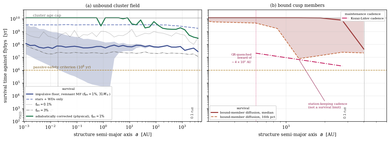
We quantify the cumulative hazard with a Monte Carlo over encounter statistics (Figure 1; method and parameters in the Appendix; code in the paper repository, paper/figs/fig1_envelope.py): impact parameters from the focused distribution of Eq. 4 within b < 30a, relative speeds drawn as described in the Appendix, impulsive kicks with the saturated form above, and dynamical survival defined as eccentricity random-walking to orbit-crossing (e ~ 0.5). The perturber mass function has two stellar components (main sequence plus white-dwarf tail) and, because kick variance scales as m_★² and mass segregation concentrates heavy remnants inside the influence radius, a segregated remnant extension: neutron stars (1.4 M_☉, 2 per cent number fraction) and stellar-mass black holes (10 M_☉) at a fiducial local number fraction of 1 per cent, bracketed by 0.1 and 3 per cent. The bracket is anchored to the retained core black-hole populations of the González Prieto et al. (2025) growth models, whose global fractions are of order 0.1–1 per cent, enhanced centrally by segregation. The calculation remains conservative in omitting adiabatic suppression.

The result is structurally simpler than the constraint inventory led us to expect: flybys never set the outer boundary, but the remnant tail controls the lifetime normalization. The median impulsive-diffusion lifetime is roughly flat from 10⁻³ to 4×10³ AU, because the kick variance per encounter and the encounter rate scale inversely (⟨δ²⟩ ∝ a⁻¹ from the saturated penetrating passages that dominate it, Γ ∝ a in the focused regime), so their product is scale-free. Its value is ~3×10⁹ yr for the stars-plus-WDs function alone, dropping to ~1.5×10⁹, ~5×10⁸, and ~1.5×10⁸ yr at black-hole fractions of 0.1, 1, and 3 per cent: a 10 M_☉ perturber at even 1 per cent number fraction multiplies the kick variance several-fold. The earlier draft’s claim that the floor is comparable to the cluster age does not survive the remnant correction; the defensible statement is that the passive floor is a few ×10⁸ yr at the fiducial remnant fraction, with an envelope floor of ≈10⁸ yr at the most pessimistic remnant fraction explored (a min-of-bins statistic with seed-to-seed spread of ~0.9–1.1×10⁸ yr; Appendix), and exponentially lengthened by adiabaticity at depth.

The Bahcall–Wolf cusp bracket. The Monte Carlo uses the core-average perturber density; a relaxed bound cusp around the hole would raise it locally, and the correction is large enough to state as a bracket rather than a note. The existence question comes first. A relaxed cusp requires the stellar system inside the influence radius to have completed energy relaxation; ω Cen is not core-collapsed and its core relaxation time is ~10 Gyr, so a fully relaxed cusp is marginal, and whether the González Prieto et al. (2025) N-body realizations develop one is checkable and is the decisive test. If a cusp exists, the heavy species follow n ∝ r^−7/4 (Bahcall & Wolf 1976, 1977): at the envelope edge, 0.1 r_infl, the density rises by 10^1.75 ≈ 56 over the influence-radius value, while cusp members there move at the Keplerian ~67 km s⁻¹ rather than the 30 km s⁻¹ the Monte Carlo samples. With the diffusion coefficient scaling as n⟨m_★²⟩/v, the floor degrades by ~25×, to ~2×10⁷ yr at the envelope edge. The correction is edge-dominated and granularity-limited, however: N(<r) ∝ r^5/4 puts only ~40 cusp objects inside the stripping radius and fewer than one expected inside ~2×10² AU, where continuous-diffusion language fails and the few bound members are near co-rotating, so the deep envelope keeps its long (adiabatically protected) lifetime and the flat lifetime profile breaks at the edge rather than dropping uniformly. The defensible statement of the floor is therefore a bracket: ~5×10⁸ yr with no cusp, degrading to ~2×10⁷ yr at the envelope edge under a fully relaxed cusp.

The survival criterion itself needs a second clock. The e = 0.5 threshold marks dynamical death, when swarm orbits cross and membership is lost; an unmaintained swarm dies operationally much earlier, because differential kicks pump internal velocity dispersion, and once neighboring orbits cross at their much smaller spacing (Δa/a ~ 10⁻³ for a dense swarm) the collisional cascade of Section 3.3 begins. Scaling the random walk to that threshold gives a grinding-onset time of (e_swarm/e_cross)² ≃ 4×10⁻⁶ of the diffusion floor, ≈2×10³ yr at the fiducial floor: of order 10³ yr, consistent with the abandonment timescale derived independently in Section 3.3. The two clocks are reconciled by maintenance: the station-keeping needed to null the accumulated differential drift is a small trim budget (the per-encounter kicks are Δv ≲ cm s⁻¹ against orbital velocities of 10²–10³ km s⁻¹), but it is strictly required. Passively bound is not passively functional, and every long-lived swarm in this paper is a maintained swarm. The operative outer boundary remains the cluster stripping radius of Section 2.3, ~0.1 r_infl ~ 4×10³ AU, with the flyby Monte Carlo setting the maintenance-free lifetime interior to it.

2.5 The envelope

Combining Sections 2.2–2.4: for the fiducial system, engineered swarms (symmetric or phase-agnostic, per the precession constraint) persist passively from r ≃ 10² r_g (2×10⁻² AU, fueled) or r_ISCO (dormant) out to the cluster stripping radius ~4×10³ AU, with a flyby-diffusion floor of ~5×10⁸ yr at the fiducial remnant fraction (3×10⁹ yr without remnants; ~2×10⁷ yr at the envelope edge under the relaxed-cusp case of Section 2.4) and exponentially longer protected lifetimes at depth. Beyond the stripping radius, orbits bound to the hole are not durable and only cluster-orbiting architectures (outside this paper's scope) remain.

Two corollaries matter downstream. First, the thermodynamically favored location (deep, near the flow) is also the dynamically safest, doubly so once adiabatic protection is counted: the environment does not penalize the architecture Paper A's physics prefers, a nontrivial consistency check the hypothesis could have failed. Second, the envelope concentrates any engineered mass within ~4×10³ AU ~ 10⁻¹ r_infl of the hole, with the thermodynamic gradient pushing occupation deep into the arcsecond-unresolvable interior: observable only through its energetic and dynamical residue, the subject of Section 3.

2.6 Hazards beyond flybys

Three further environmental processes deserve quantitative treatment. Each is a candidate defeater; none defeats, though the first comes closest.

Tidal disruption events. A cluster-core IMBH tidally disrupts stars scattered into its loss cone. Rates for IMBHs in evolved globular clusters, computed with loss-cone methodology of the kind developed for the supermassive case (Stone & Metzger 2016), are ~10⁻⁸–10⁻⁷ yr⁻¹ per cluster for main-sequence stars, with white-dwarf disruptions rarer by a factor of ~30–100. During a disruption the accretion luminosity approaches Eddington, sustained for months to years of fallback: the flux at r = 1 AU is ~10⁹ times the solar constant, and no plausible material hardening survives it in place. Feasibility therefore requires that a TDE be survivable by response rather than endurance: loss-cone stars are in principle identifiable and trackable long before disruption, and the months-long fallback rise gives further warning, so temporary evacuation outward along the envelope, or shadowing at large inclination, is an engineering requirement we impose on any architecture rather than a reason to exclude one. The expected recurrence time of ≳10⁷ yr sets the natural amortization horizon of the installation: a 10⁸–10⁹-yr occupation must plan for several such events. The TDE duty cycle also reconciles engineered occupation with the present silence at no extra cost: post-TDE fallback outshines any steady configuration for ~10²–10³ yr per ~10⁷-yr recurrence, a duty cycle of ≲10⁻⁴, so catching ω Cen mid-flare was never likely under any hypothesis. And TDEs cut the other way, as an observational gift: any future TDE flare in ω Cen both confirms the hole and activates the variability channel of Section 3.2 at high signal-to-noise, and the framework of Section 4 treats a TDE with anomalous light-curve regulation as one of the few single-epoch events that can move ln K substantially.

Black-hole wander. The hole is a Brownian particle in the stellar bath: N-body characterizations give r.m.s. displacements of order 10⁻²–10⁻¹ pc for 10³–10⁴ M_☉ holes in ω Cen-like cores, with wander amplitude scaling inversely with hole mass. For the fiducial 2×10⁴ M_☉ hole the expected wander is ≲10⁻² pc ~ 2×10³ AU: comparable to the 4×10³ AU envelope. Structures bound to the hole simply ride along (the swarm orbits the hole, and hole plus swarm wander together through the cluster), so wander does not threaten the installation; what it threatens is the observer's astrometry, since the kinematic center and the hole need not coincide at the 10⁻²-pc level. Paper C's astrometric programs already marginalize over center position; the wander amplitude is itself mass-dependent and therefore carries independent information about M in long-baseline proper-motion data.

Gas drag and erosion. ω Cen retains a measurable intracluster medium: central ionized densities n_e ~ 0.1–0.3 cm⁻³. Ram-pressure drag on a swarm element at the deep-envelope orbital velocity (a few ×10³ km s⁻¹; 4×10³ km s⁻¹ at the 1 AU fiducial) removes a fractional momentum ≲10⁻⁶ per kyr at the measured densities: negligible. Sputtering and dust impacts are similarly small in an old cluster with no star formation and depleted debris populations. Gas matters for fuel, however, the next subsection.

2.7 The fuel budget

The Blandford–Znajek architecture of Paper A needs mass supply, and the measured medium bounds it. Bondi accretion from gas of density n_e ≃ 0.23 cm⁻³ at relative velocity ~σ gives

about 10⁻⁴ of the Eddington rate. Two caveats bound this from both sides. It is an upper bound insofar as the density at the hole's actual location may be below the cluster mean: the accretion non-detections are consistent with the hole occupying a locally evacuated region, and the Bondi radius (~GM/c_s² ~ 2×10⁵ AU) samples gas the surveys average over. It is a lower bound insofar as it ignores harvesting: stellar winds from the ~10³ giants inside the influence radius, or deliberately imported mass, can raise supply by orders of magnitude at the cost of visibility. At MAD-plus-spin effective efficiencies of order unity, realized only at high spin (η_jet ≃ 1.4 at a_★ ≃ 0.99, falling roughly as a_★² to a factor ~5 lower at a_★ = 0.5; Paper A), the ambient rate gives extractable power P ~ Ṁ_Bc² ≃ 3×10³² W ≃ 8×10⁵ L_☉, with the fuel ceiling carrying the same η(a_★) dependence: the ambient medium alone, with no harvesting of stellar winds or imported fuel, funds a computational budget two orders of magnitude above the waste-heat ceiling derived in Section 3.1.

That headroom assumes the Bondi rate reaches the horizon, and in natural hot, low-Eddington flows it does not: the inflow declines inward, Ṁ(R) ∝ R^s with s ≃ 0.3, as most of the captured gas is unbound into outflows (Blandford & Begelman 1999; Yuan & Narayan 2014). Over the nine decades from the Bondi radius (r_B ≃ 1.8×10⁵ AU) to r_g, the suppression is (r_B/r_g)^0.3 ≈ 500, giving P_fuel ≃ 1.6×10³ L_☉; adopting instead the empirical Sgr A* figure of ~1 per cent of the Bondi-radius rate gives ≃8×10³ L_☉. Either value lands at or below the warm-swarm waste-heat ceiling of Section 3.1, so for a natural flow the supply and concealment constraints bind together, and the "supply never binds" ordering holds only for the engineered case. The engineered case is available, and it unifies two of this paper's results: a system drawing more than the ADIOS-suppressed rate is a system that has suppressed its own outflow, and that is the same control action, regulating horizon magnetic flux and mass supply, that produces the low-R variability deficit of Section 3.2. The fuel budget and the R statistic are two faces of one control action. We therefore carry both cases through the paper: natural-suppressed (P_fuel ~ 10³–10⁴ L_☉) and engineered-unsuppressed (P_fuel ≃ 8×10⁵ L_☉), with the Appendix-B prior ceiling stated for the pair.

For an installation with outflow control, then, the binding constraint on a present-day ω Cen system is thermal (getting rid of entropy without detection), never supply; without it, the two constraints meet. The unsuppressed ordering is a nontrivial output: for stellar-mass holes in the same environment the two constraints reverse even in the engineered case, an independent reason the hypothesis family selects IMBHs. The same numbers close the loop on the accretion non-detection: the deep ATCA and JWST limits require the natural radiative efficiency of any Bondi-fed flow to be ≲4×10⁻³, uncomfortable for the quiescent-IMBH null at the upper end of the mass range and what an engineered-occupation flow predicts for output extracted as work rather than radiation. The adjudication in Section 5 prices this observation for both hypotheses rather than letting either claim it informally.

3. Observable residue

3.1 Waste-heat floor

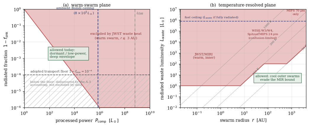
Paper A argued that horizon entropy disposal permits computation with radiated waste heat far below the Dyson-sphere expectation. Here we make the floor quantitative, and we first fix the bookkeeping, because the mainstream position is an energy-conservation argument: Curtis et al. (2026) state that Dyson-scale computation must reradiate nearly all of the energy it absorbs, making mid-infrared thermal emission the robust technosignature. The horizon-sink architecture disputes that position at the level of energy conservation itself, not merely entropy accounting. Let P_comp be the power processed by the swarm and f_sink the fraction of the waste energy delivered across the horizon rather than radiated; the entropy rides with its carriers, so a single fraction serves for both. Energy beamed across the horizon is not reradiated at all: it adds to M, and since T_H ∝ M⁻¹ the disposal channel deepens as it is used, a weakly self-improving property. What must be radiated is only the missed fraction, L_waste = (1 − f_sink) P_comp, re-emitted thermally at the temperature set by the swarm radius. For single-sided radiators at unit covering fraction, T_eff ≃ (L_waste/4πr²σ_SB)^1/4: 1 L_☉ at r = 1 AU gives 394 K, 1 L_☉ at 10³ AU gives 12.5 K, and a 50 K swarm at 10³ AU corresponds to L_waste ≈ 160 L_☉. This T_eff(r) assumes unit covering fraction with single-sided radiators; a sparse swarm of covering fraction f_cov runs hotter by f_cov^−1/4, moving mass into the JWST wedge and shifting the composite ln K of Section 5 to −0.34 at f_cov = 10⁻², inside the quoted band.

The engineering limit on f_sink is transport: waste energy must be carried inward, against the swarm's own power draw, by mass flux or directed radiation into the horizon. The capture-cone and étendue accounting of Appendix A.3 bounds 1 − f_sink ≳ 10⁻⁴ for swarm architectures within the envelope, set by the fraction of beamed power unavoidably intercepted and re-thermalized by swarm elements along the transport path. The sign of its influence is worth stating: a lower true floor (better beaming than the A.3 accounting allows) weakens the mid-infrared charge against engineered occupation and moves ln K toward zero, while a higher floor tightens the P_comp ceiling and strengthens it (Section 6.1). The floor is therefore

Converting that floor into a P_comp bound requires a temperature axis, because which instrument limits L_waste depends on where the thermal emission peaks. The deep JWST limits at the kinematic center constrain warm sources: a swarm at r ≲ a few AU re-radiates at T_eff ≳ 150 K, peaks within MIRI coverage, and inherits the sub-L_☉ point-source limit, giving P_comp ≲ L_lim/(1 − f_sink) ≲ 10³–10⁴ L_☉. A cool outer swarm evades it: at r ~ 10²–10³ AU the emission peaks at 20–60 μm and beyond, where the operative limits are WISE W3/W4 and Spitzer/MIPS photometry whose 6–18 arcsec beams are confusion- and crowding-limited in the ω Cen core, weakening the effective point-source bound to ~10² L_☉, and past 60 μm (MIPS 70 μm only) to ≳10⁴ L_☉. The single-number bound of an earlier draft implicitly assumed the warm case; the defensible statement is radius-dependent, and the Appendix-B adjudication now marginalizes over swarm radius accordingly. An engineered system operating at the radius-appropriate ceiling is consistent with all current data; deeper MIR photometry tightens the warm wedge linearly, while the cool wedge waits on far-infrared sensitivity. Figure 2 assembles the warm-swarm plane and the temperature-resolved plane, with the transport floor and the fuel ceiling of Section 2.7, into the constraint space that defines the surviving engineered-occupation parameter volume.

3.2 The MAD-regulation signature

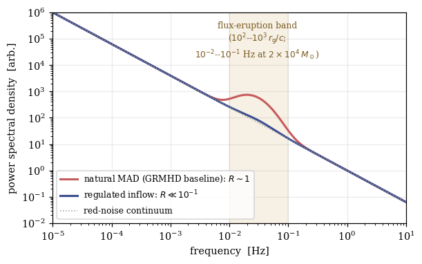
The second channel is new to this paper. General-relativistic magnetohydrodynamic simulations establish that natural accretion in the magnetically arrested state is intrinsically episodic: magnetic flux accumulates at the horizon, chokes the inflow, and erupts in quasi-regular flux-expulsion events, producing characteristic variability in jet power and radiative output with a MAD > intermediate > SANE hierarchy in both luminosity and its variance. The eruption mechanism is plasmoid-mediated reconnection of the accumulated horizon flux, resolved ab initio by Ripperda et al. (2022), whose flare cycle of ~10²–10³ r_g/c between flux accumulation and expulsion is the recurrence we adopt; the state-resolved variability tables of the 2026 GRMHD compilation place the MAD eruption power in the same interval at matched mean luminosity. For M = 2×10⁴ M_☉ that cycle is ~10–10² s, comfortably within the cadence of X-ray monitoring.

A system engineered for steady power extraction has an incentive absent in nature: eruptions are interruptions. Regulating the delivered mass and flux (the control variable identified by the simulations is horizon magnetic flux itself) suppresses the eruption cycle and its variability signature. We therefore forward-model the residue as a variability deficit: an accreting IMBH whose X-ray (or optical) power spectrum lacks the flux-eruption band that GRMHD baselines predict for its luminosity and inferred state. Quantitatively, we define the regulation statistic R as the ratio of integrated power in the eruption band (10⁻²–10⁻¹ Hz for the fiducial mass) to the GRMHD-calibrated expectation at matched mean luminosity; natural MADs populate R ~ 1 with factor-of-few scatter, and R ≪ 10⁻¹ sustained over many cycle times has no identified natural mechanism (Figure 3). The band edges follow directly from scaling the Ripperda et al. (2022) flare cycle of 10²–10³ r_g/c to M = 2×10⁴ M_☉ (r_g/c = 0.1 s, hence 10–100 s), with the 2026 GRMHD state tables placing the eruption power in the same interval; an earlier draft extended the band a decade lower, which nothing in the cited cycle supports. The main confusion risk in applying the statistic is contamination from the intermediate magnetic state, whose eruption power is partially suppressed relative to MAD, so the baseline must be conditioned on the inferred state, never on luminosity alone.

Two instrument realities shape where R can be measured. First, at the fiducial mass R is an X-ray/optical statistic; radio is excluded twice over. Synchrotron self-absorption in any compact GHz-emitting flow puts the τ = 1 photosphere at ~10²–10⁴ r_g, low-pass filtering intrinsic variability at Δt ≳ 10–10³ s, directly on top of the eruption band, so a radio non-detection of the band is expected under the quiescent and engineered hypotheses alike and carries no discriminating power. Interstellar scintillation compounds the problem: a microarcsecond-scale source at 5.4 kpc scintillates at GHz frequencies on minutes-to-hours timescales, adding modulation uncorrelated with accretion in and near the band, so even a genuinely regulated (low-R) source would show a measured R biased upward unless the scintillation is modeled out. Second, the statistic has a detectability threshold. Distinguishing R ~ 1 from R < 0.1 requires several counts per ~10 s cycle sustained over many cycles, i.e., F_X ≳ a few ×10⁻¹² erg cm⁻² s⁻¹ for m²-class effective area, corresponding to L_X ≳ 10³⁴–10³⁵ erg s⁻¹ ≈ 10⁻⁸–10⁻⁷ L_Edd at the fiducial mass. The channel therefore activates in flare and TDE states rather than in deep quiescence, which is consistent with the TDE-as-gift framing of Section 2.6: the events that confirm the hole are the events bright enough to measure R.

The signature has three properties valuable for adjudication. It is conditional: it activates only if accretion is ever detected, so it presently constrains nothing (ω Cen's hole is electromagnetically silent). It is differential: it compares a source against a physics baseline at matched parameters, canceling many systematics. And it is disprovable in place: detection of normal flux-eruption variability from a future ω Cen accretion flare would count against engineered occupation in the framework below, making the channel one of the few that can move evidence in both directions.

3.3 Relic residue: the abandoned swarm

Persistence is conditional on maintenance, and prior work on megastructure collisional cascades has shown what maintenance failure means: once guidance fails, swarm elements collide, and a collisional cascade grinds the population to dust on a timescale of roughly the orbital period divided by the covering fraction. The deep envelope makes this dramatic. At r ~ 1 AU around the fiducial hole the orbital period is ~3 days; for covering fractions 10⁻⁴–10⁻² the first-collision timescale ~ P/f_cov is years to decades, and the full cascade completes on a timescale of order 10³ yr, orders of magnitude faster than for stellar-orbit megaswarms and consistent with the grinding-onset clock of Section 2.4. The end state differs too, and the difference is observationally decisive: cascade debris around a star settles into a long-lived warm dust population, a passive relic technosignature, whereas debris around a black hole is progressively drained, its periapsis distribution fed toward the loss cone by continuing collisions and flyby perturbations and its finest grindings coupled to whatever gas flow exists; the drainage rate remains an estimate, qualified in Section 6.1. The hole removes its own debris. An abandoned engineered-IMBH system therefore passes through a brief bright phase (cascade grinding plus enhanced accretion luminosity as debris drains) and then reverts to a naked quiescent hole, indistinguishable from the gas-starved null except possibly through spin.

Three consequences follow. First, a fourth hypothesis joins the menu at zero structural cost: a formerly engineered, now-abandoned system, whose observables today equal the gas-starved quiescent null plus high spin, and whose prior couples to the goal-stability open problem flagged in Paper B. Second, the searchable relic window is short, so population-level searches for dead installations have low yield around IMBHs specifically; non-detection of relic dust in ω Cen carries almost no evidence either way, and the framework scores it accordingly. Third, spin becomes the only durable fossil, and an objection must be met before relying on it: Blandford–Znajek extraction spins the hole down, and MAD jets remove angular momentum faster than accretion supplies it, so one might expect long use to erase the very fossil we propose reading. The rates rescue the argument: in the MAD spin-down calculus, the spin-down per unit accreted mass is of order |Δa_★| ~ ΔM/M, so erasing a high spin requires cycling a mass comparable to the hole's own through the flow, and at the ambient fueling of Section 2.7 that takes M/Ṁ_B ~ 4×10¹¹ yr. Only a civilization importing mass at far above ambient rates for ≫10⁹ yr would measurably despin the hole, and that regime is separately excluded by the waste-heat ceiling.

What spin discriminates deserves a more careful statement than our earlier draft gave it. The natural expectation is a channel mixture, set by growth history rather than by any single attractor: repeated comparable-mass mergers drive χ toward the ≃0.7 attractor (Fishbach, Holz & Farr 2017; Gerosa & Berti 2017); gas-poor growth by minor mergers and inspirals of isotropically arriving compact objects random-walks the spin to low values, a_★ ~ 0.1–0.3; and prolonged coherent disk accretion spins the hole up toward the radiation-limited maximum a_★ = 0.998 (Bardeen 1970; Thorne 1974). The González Prieto et al. (2025) models constrain which growth channels operated in ω Cen (we cite them for growth history only; they do not track spin), and a hierarchical-merger-dominated history would land near 0.7, uncomfortably close to the engineered high tail. The discriminating contrast is therefore ≃0.7 versus ≳0.9, sharper than low-versus-high but weaker than the "moderate versus high" framing of earlier drafts: a LISA-era spin measurement moves ln K substantially only if it lands outside the merger attractor's scatter. The information forecast of Section 5 inherits this reduced weighting.

3.4 EMRI dephasing: the mass channel

Every residue channel above constrains power, variability, or spin. One channel constrains engineered mass, and it comes for free with the gravitational-wave observation the series already relies on. Matter in the vicinity of an inspiral imprints secular phase shifts on the waveform; the environmental-effects literature for extreme- and intermediate-mass-ratio inspirals, founded by Barausse, Cardoso & Pani (2014), quantifies how accretion disks, dark-matter spikes, and other mass distributions dephase an inspiral over an observation. An engineered swarm is a mass distribution like any other. If a stellar-mass compact object is ever caught inspiraling into the ω Cen hole, the waveform is a scale: it weighs whatever hardware shares the inspiral's neighborhood, independent of that hardware's luminosity, temperature, or duty cycle.

The channel's reach must be stated carefully, because it is short. The secular dephasing from an exterior axisymmetric mass falls as (r_orb/r_torus)³ per orbit, so a debris torus or swarm at 10²–10³ AU accumulates negligible phase against an inspiral at ~10⁻³–10⁻² AU; we make no claim of debris-torus reach, and the channel does not repair the relic-searchability gap of Section 3.3. What it constrains is mass at or inside the inspiral track, r ≲ 10⁻² AU, and that limitation is well matched to the hypothesis: Paper A's thermodynamic gradient concentrates hardware at exactly those depths, and the envelope of Section 2 permits it there. A LISA-band inspiral through an occupied deep envelope would traverse the swarm itself. An order-of-magnitude scope for the fiducial system: an inspiral accumulates ~10⁵–10⁶ radians of orbital phase over a multi-year observation, and matched filtering resolves phase drifts of order unity, so fractional perturbations at the 10⁻⁶–10⁻⁵ level in the enclosed mass along the track are in principle measurable, a sensitivity to swarm masses far below any other channel's floor. Turning that scope into a forecast requires real waveform modeling, including the degeneracies with the astrophysical environmental effects already cataloged in the literature; we defer that calculation, and any figure it would support, rather than publish an unmodeled curve.

Two properties carry into the adjudication. The channel is two-sided, like R: a measured vacuum inspiral, dephasing consistent with zero environmental mass, counts against engineered occupation at the depths the hypothesis most values, and the framework of Section 4 scores it accordingly. And it inherits the spin channel's schedulability problem: ω Cen's own IMRI probability is ~10⁻⁹–10⁻⁶ yr⁻¹ (Section 5), so the channel is population-level, a constraint LISA accumulates across the Galactic IMBH census rather than a scheduled ω Cen observation. It enters the information forecast of Section 5 as the fourth channel on those terms.

3.5 Predicted-signature table

Table 1 summarizes what each channel looks like under the engineered hypothesis and the two astrophysical nulls defined in Section 4.1.

The table exposes the central inferential difficulty, stated plainly in Paper A and now quantified: silence is predicted by everything. The engineered and quiescent-IMBH hypotheses are near-degenerate in every electromagnetic channel while the system is dormant. The channels that separate them are spin (engineered selection favors a_★ ≳ 0.9; natural growth favors the channel mixture of Section 3.3, whose merger attractor at χ ≃ 0.7 limits the contrast), the R statistic (active only during accretion episodes above the Section 3.2 threshold), EMRI dephasing (active only if an inspiral occurs; Section 3.4), and the waste-heat floor (which separates them only near the sensitivity ceiling). This degeneracy structure, rather than any single measurement, is what the adjudication framework must manage.

4. The adjudication framework

4.1 Hypothesis space

We adjudicate among three hypotheses about the ω Cen center:

The menu is explicit and extensible; adding hypotheses (an exotic compact object, instrumental systematics on the fast stars, the abandoned-system variant of Section 3.3) changes bookkeeping, never structure. The abandoned-system variant is degenerate with the quiescent-IMBH null on every current channel (Section 3.3) and is therefore not separately scored until a spin measurement exists. We follow the convention that H_eng is reported only as odds against the best-performing null, never against a strawman.

4.2 Per-messenger Bayes factors

For each observational channel i with data d_i, the Bayes factor between hypotheses H_a, H_b is

with channel likelihoods built from the forward models of Section 3 and, following radio-SETI practice, an explicit interference/systematics component mixed into every likelihood so that "instrumental artifact" is priced inside each channel rather than adjudicated informally afterward. Priors on H_eng parameters are pre-registered (Appendix, §B) and varied over stated ranges in sensitivity analysis; the framework's outputs are always reported as (odds, prior-sensitivity band) pairs, never as bare odds.

4.3 Cross-messenger combination

Channels are combined multiplicatively where independent, K_tot = ∏_i K_i, with two corrections imported from gravitational-wave counterpart methodology. First, a coincidence term: hypotheses that predict correlated anomalies across channels (as H_eng does for MIR excess and low R during an accretion episode) earn a likelihood contribution from the observed coincidence structure itself, computed from the joint forward model rather than the product of marginals. Second, an independence audit: channels sharing calibrators, atmospheric paths, or reduction pipelines are grouped and their shared systematics marginalized jointly before multiplication. Both corrections are conservative in effect: the coincidence term rewards only pre-registered correlation patterns, and the audit only ever weakens evidence.

4.4 Decision thresholds

We adopt a logarithmic odds scale with pre-registered action bands, stated here for ln K of H_eng over the best null:

Two design points. The "candidate" band requires multi-messenger support by construction, honoring Paper C's two-messenger rule; no single channel, at any significance, can reach it, because single-channel anomalies are where every historical false alarm has lived. And the kill conditions of Paper A map onto the same scale in the other direction: the pre-registered falsifiers (e.g., LISA measurement of low spin; resolution of the mass tension in favor of H_sub) enter as ordinary likelihood terms and drive ln K negative, so confirmation and falsification run through one pipeline rather than two standards. The framework is deliberately instrument-agnostic: nothing in Sections 4.2–4.4 references ω Cen, and the machinery applies unchanged to any technosignature target with a defined null menu.

5. Worked example: Omega Centauri today

We now run the current ω Cen data through the framework. Inputs: the fast-star kinematics, the N-body modeling, the MSP timing bound (with the TRAPUM 2026 mass limit), the deep radio silence, and the JWST infrared limits. The computation implements the Appendix-B model (deliberately minimal: radius-marginalized hard-threshold MIR likelihood, log-flat priors, 2×10⁶ prior draws); code in paper/figs/fig3_lnk.py, results in Figure 4.

• Quiescent IMBH vs. remnant subcluster: the interesting contest, and the framework's finding is that it is currently a stand-off dominated by the kinematics-versus-timing tension: the fast stars pull toward a point mass, the pulsars toward an extended one, and the combined |ln K| is ≲1 with sign depending on how the two datasets' systematics are weighted. As an independent check, the imbh-constraints aggregation engine of the series' public toolchain, run on its nine-constraint curated compilation, returns an empty jointly-allowed mass window (formal tension verdict: the kinematic floor exceeds the tightest model-dependent ceiling), confirming that no point-mass value satisfies all published constraints at face value. The framework adds discipline, and no verdict, to a tension the community already knows; per series policy the tension is recorded, never collapsed.
• Engineered vs. best null: ln K sits in the null-favored band, as it should. The only active channel today is waste heat, and, with the likelihood marginalized over swarm radius against the radius-dependent instrument limits of Section 3.1, it yields ln K = −0.29 at fiducial priors (prior-sensitivity band −0.59 to −0.05 as the dormancy prior runs from 0.1 to 0.9): the electromagnetic silence sometimes informally cited as consistent with engineering is, in the accounting, mildly against engineered occupation, because the mid-infrared limits exclude the ~50 per cent of the active-installation prior volume that is warm or luminous enough to detect, while every other channel is inactive or degenerate and contributes nothing. The radius marginalization matters: against the warm-swarm limit alone the same computation gives ln K = −0.40, so accounting for cool outer configurations moves the verdict toward zero. The leak prior's lower bound is an engineering estimate (Section 3.1, Appendix A.3): repeating the computation with the prior extended down to 1 − f_sink = 10⁻⁶ gives ln K = −0.20 instead of −0.29, so a softer transport bound softens the conclusion without reversing it. A second sensitivity is the fuel ceiling: the fiducial prior extends P_comp to the unsuppressed 7.6×10⁵ L_☉, and truncating it at the ADIOS-suppressed natural ceiling of Section 2.7 (~10³ L_☉) removes most of the detectable prior volume, moving the mid-infrared ln K toward ≈−0.1 (Appendix B). More important than either sensitivity is what dominates the total: the present evidence budget is set by the dormancy prior (the data enter only through P(quiet | active) = 0.50), so the framework's present value is the forecast, not the number. The surviving configurations are dormant or low-power, deep-envelope systems (Figure 2). Quantifying that shrinkage is the point; the hypothesis pays for its unfalsified survival in measured parameter volume.
• Information forecast: ranking the Paper C programs by expected |Δln K| per unit cost, the leaders are (1) resolution of the mass tension by continued MSP timing plus Gaia DR4 astrometry, which arbitrates the two astrophysical nulls and thereby moves the engineered hypothesis's denominator; (2) any detection of accretion at any level, which activates the R statistic, the only cheap channel with large discriminating power in both directions; (3) the LISA-era spin measurement, still the largest potential mover though with the contrast reduced to ≃0.7 versus ≳0.9 by the merger attractor (Section 3.3), and the least schedulable: intermediate-mass-ratio inspiral rates per IMBH are ~10⁻⁹–10⁻⁶ yr⁻¹, so ω Cen yielding its own inspiral during the mission is unlikely and the spin constraint will more probably arrive statistically, from the population of ω Cen-like systems LISA does catch, than from ω Cen itself. The relic analysis of Section 3.3 raises the stakes on this channel: spin is the one fossil that survives abandonment, so the LISA-era population measurement adjudicates the engineered-history hypotheses for the whole Galactic IMBH population at once, and the per-target frameworks of this paper compose naturally into that population-level test. A fourth channel now joins the forecast: (4) EMRI/IMRI environmental dephasing (Section 3.4), the only channel constraining engineered mass, which shares the spin channel's LISA-era timing and schedulability and, like R, moves evidence in both directions, since a vacuum inspiral counts against engineered occupation at the depths the hypothesis most values. Deeper radio silence, by contrast, now moves ln K weakly for every pairing: for this hypothesis menu the existing limits are already deep enough that further depth buys little discrimination.

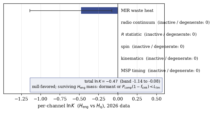
6. Discussion

6.1 Limitations

The feasibility envelope depends on cluster-center parameters that carry real uncertainty (mass function of the remnant tail; central density profile inside the influence radius, whose bound-cusp case is bracketed analytically in Section 2.4 rather than run through the Monte Carlo) and on a material-strength scale taken from present technology; both are varied in the Appendix. The two largest levers are the remnant tail, which moves the flyby-diffusion floor by an order of magnitude across the explored 0.1–3 per cent black-hole fraction bracket (Section 2.4), and the cusp existence question, worth a factor ~25 at the envelope edge and resolvable by inspecting the González Prieto et al. (2025) realizations; the remaining parameters move the boundaries by factors of a few. The MAD-regulation channel inherits the systematic uncertainties of the GRMHD baseline literature, which is simulation-calibrated rather than observationally calibrated at IMBH masses. The adjudication framework shares the standard vulnerability of Bayesian model selection to unmodeled hypotheses: it ranks the menu it is given, and a surprise outside the menu (an astrophysical mechanism not yet imagined) would be mis-scored until added. The mitigation is procedural rather than mathematical: the menu is public, extensible, and versioned.

Two numbers used above deserve explicit qualification at the claim level.

The transport floor. The geometric content of the bound 1 − f_sink ≳ 10⁻⁴ is now a calculation (capture cone, beaming gain, étendue, and the plasma-cutoff carrier condition; Appendix A.3); what remains estimated is the re-interception term, the covering-fraction floor on power re-thermalized within the swarm, which a full radiative-transfer treatment of the swarm interior would replace. Its influence on the adjudication is bounded and signed: extending the leak prior down to 10⁻⁶ moves ln K from −0.29 to −0.20, well inside the dormancy-prior band of [−0.59, −0.05], so no conclusion of Section 5 turns on the exact value.

The drainage timescale. The ~10³ yr figure of Section 3.3 is an estimate. The asymmetry it rests on is robust, since relic dust persists around a star while debris around a hole is fed toward the loss cone and removed, but the rate is not. Closing that gap requires a loss-cone refill calculation for the debris population, tracking collisional periapsis diffusion and the coupling of the finest grindings to the ambient flow; we state the gap rather than supply a number that calculation has not yet produced.

6.2 Relation to the series and beyond

Within the series, this paper closes the constructive quadrant: Paper A argued the destination is attractive, and Section 2 finds the destination is habitable by infrastructure, with the thermodynamically preferred region also the dynamically safest. It also arms Paper C's campaign with the scoring machinery its two-messenger policy presupposed, and returns to Paper D a refined survival input (p_s now decomposable into transit and residence terms, the latter bounded here). One dependency flag on that export: the residence-survival figure Paper D imports (≈0.8 over 10⁸ yr) is derived from the no-cusp diffusion floor and moves under the relaxed-cusp case of Section 2.4, so Paper D's fiducial should carry the same bracket. Beyond the series, the two exportable products are the envelope method, applicable to any proposed megastructure environment with a stated perturber population, and the adjudication framework, applicable to any technosignature program willing to pre-register its nulls.

6.3 Conclusion

The engineered-IMBH hypothesis survives its first engineering audit and its first quantitative adjudication, in both cases by narrowing: infrastructure persists only within ~4×10³ AU of the hole, and the surviving parameter space after current data is dormant, low-power, and deep. Every forthcoming measurement listed in Section 5 shrinks it further or breaks it open. Either outcome is progress that a hypothesis without an envelope, a residue model, and a scoring rule could not deliver.

7. Appendices: Monte Carlo, priors, reproducibility

A. Flyby Monte Carlo: method and parameters

Method (implemented in paper/figs/fig1_envelope.py; fixed seed 20260717). For each of 40 logarithmic radius bins a ∈ [10⁻³, 4×10³] AU: (1) 2×10⁵ encounters are drawn with impact parameter from the gravitationally focused cumulative distribution Q(b) ∝ v_rel²b² + 2GMb truncated at b_max = 30a (contributions beyond carry <10⁻³ of the kick variance), relative speed drawn as v = 0.3σ + x with x a Rayleigh variate of scale σ = 21 km s⁻¹, i.e., a Rayleigh distribution shifted upward by 0.3σ (mean 1.25σ + 0.3σ = 1.55σ; the JSON output of Appendix C records the exact parameterization), below the Maxwellian relative-speed mean of ~2.26σ; since slower encounters deliver larger kicks, the choice is conservative for swarm survival, and mass from the perturber mass function. The baseline function has two stellar components (0.35 M_☉ with weight 0.7; 0.6 M_☉ white-dwarf tail with weight 0.3); the fiducial function adds segregated remnants, 1.4 M_☉ neutron stars at number fraction 0.02 and 10 M_☉ black holes at number fraction f_BH ∈ {0.001, 0.01, 0.03} with the stellar weights renormalized, at fixed total number density. (2) Each encounter contributes an impulsive eccentricity kick δ = 2(m_★/M) min[1,(a/b)²](v_orb/v), i.e., δ = δv_tid/(2v_orb) with the O(1) geometric coefficient set to unity; that choice sits on the optimistic side by a factor of ~2 in the δ² timescale, offset by the conservative velocity sampling above and by the neglect of adiabatic suppression, so the net sits within the stated factor-few accounting. No adiabatic suppression is applied (conservative). (3) Per history (2×10⁴ per bin), survival time is the random-walk first-passage to e = 0.5: encounters to threshold n_★ = e²/⟨δ²⟩ with CLT scatter, divided by the total encounter rate Γ(<b_max), capped at 12 Gyr. The bookkeeping is thus: the 2×10⁵ encounter draws per bin characterize the per-encounter kick-variance statistics; each of the 2×10⁴ histories then draws its encounter count analytically from that first-passage distribution rather than re-simulating individual encounters, so a history at the median spans ~n_★ ~ 10⁴–10⁶ encounters depending on bin. Single-passage disruption is impossible at these mass ratios (δ ≲ 10⁻² even for penetrating passages, ≲10⁻¹ for the rare black-hole perturbers); direct star–element scattering contributes negligibly at any realistic covering fraction. One density systematic is treated analytically rather than simulated: the calculation uses a core-average perturber density (10⁴ pc⁻³) with gravitational focusing capturing only the unbound flux, whereas a Bahcall–Wolf-type bound cusp around the hole would raise the local perturber density at 10–10³ AU. The curves here are therefore the no-cusp case; the relaxed-cusp bracket (×~25 degradation at the envelope edge, granularity-limited at depth) is derived in Section 2.4, and cusp existence is the checkable question flagged there.

Results. For the stars-plus-WDs baseline, median lifetimes are 3.4×10⁹, 3.3×10⁹, and 2.5×10⁹ yr at a = 10, 10², 10³ AU: flat, by the scale cancellation ⟨δ²⟩ ∝ a⁻¹, Γ ∝ a discussed in Section 2.4. Adding the remnant components lowers the floor in proportion to the added ⟨m_★²⟩: medians at the same radii are (1.6, 1.8, 1.4)×10⁹ yr at f_BH = 0.001, (6.5, 4.8, 4.7)×10⁸ yr at the fiducial f_BH = 0.01, and (1.9, 1.8, 1.4)×10⁸ yr at f_BH = 0.03, with envelope minima of 7.6×10⁸, 3.0×10⁸, and 1.1×10⁸ yr respectively. Varying the mean stellar mass by ×2, the density by ×3, and e_cross over 0.3–0.7 moves the floor by additional factors of a few. The earlier robustness claim must therefore be restated: across the explored remnant bracket the envelope floor is ≈10⁸ yr at the most pessimistic f_BH = 0.03. The quoted minima are min-of-noisy-bins statistics and carry ±20–35 per cent seed-to-seed variance (the f_BH = 0.03 minimum spans ~0.9–1.1×10⁸ yr across seeds), so no hard floor above 10⁸ yr is claimed. The cluster-age floor of the stars-only calculation was an artifact of the truncated mass function, and the quantitative floor is set by f_BH.

A.3: transport bound. The floor 1 − f_sink ≳ 10⁻⁴ is a calculation in three steps: delivery geometry, carrier physics, and re-interception, with only the last carrying an estimated coefficient.

Delivery. The photon-capture cross-section of the hole is σ = 27π r_g² (critical impact parameter 3√3 r_g), so from a platform at r = 10² r_g the disposal channel subtends Ω_c/4π = 6.75×10⁻⁴: isotropic emission delivers less than a thousandth of its power to the horizon, and f_sink → 1 requires a beaming gain ≳1.5×10³. That gain is optically trivial. The capture cone has half-angle θ_c ≃ 0.052 rad, so diffraction demands only an aperture D ≳ 23λ, and the étendue (concentration) limit 1/sin²θ_c ≈ 3.7×10² puts the optic area at a few hundred radiator areas. Delivery is not the binding term.

Carriers. The minimum-energy vacuum carrier, wavelength ~r_g, energy hc/r_g ≃ 7×10⁻³³ J, is a ~10 Hz wave and cannot propagate: it lies below the plasma frequency of any realistic environment (Paper A, this revision). Inside a fed envelope with n_e ~ 10⁴–10⁸ cm⁻³, ν_p ≈ 1–90 MHz, so the minimum propagating carrier energy is ≳10⁻²⁷ J, three to six decades above the vacuum figure. The delivered per-bit disposal cost is therefore set by the plasma cutoff together with dense (multi-bit-per-photon) coding up to channel capacity, and matter carriers, cold mass dropped down the capture cone, are the fallback that evades the cutoff entirely. None of this changes the geometric floor below; it fixes the cost per bit, not the intercepted fraction.

Re-interception. Beamed flux traverses the swarm on its way to the cone and is intercepted with probability of order the swarm covering fraction seen from a typical element, ≳10⁻⁴ for the covering fractions that make the swarm computationally worthwhile; the intercepted power is re-thermalized and radiated at swarm temperature. This is the binding term, and its coefficient is the one number a full radiative-transfer treatment of the swarm interior would refine (Section 6.1); the sensitivity analysis of Appendix B shows the adjudication does not turn on it.

B. Priors, likelihoods, and computation

Implemented in paper/figs/fig3_lnk.py (2×10⁶ prior draws; fixed seed). H_eng parameters: P_comp log-uniform on [1, P_fuel] L_☉ with P_fuel = 7.6×10⁵ L_☉ (the ambient Bondi ceiling of Section 2.7, quoted as 8×10⁵ in the text). That ceiling is the engineered-unsuppressed, near-extremal-spin value and is not cosmetic: it falls ~5× at a_★ = 0.5 through the η(a_★) dependence of Section 2.7, and ~10²–500× under natural outflow suppression, so a fully stated prior is a mixture over (a_★, suppressed/unsuppressed). We instead quote the sensitivity band, since the arithmetic is analytic in ln K = ln[f_d + (1 − f_d) P(quiet | active)]: at the fiducial unsuppressed ceiling, P(quiet | active) = 0.50 and ln K_MIR = −0.29; truncating the ceiling at the ADIOS-suppressed ~10³ L_☉ removes most of the detectable prior volume, raising P(quiet | active) to ≈0.8 and moving ln K_MIR to ≈−0.1; the a_★ = 0.5 ceiling sits between. Other parameters: 1 − f_sink log-uniform on [10⁻⁴, 1]; swarm radius r log-uniform over the envelope [2×10⁻², 4×10³] AU (an uninformative choice within the allowed region; the thermodynamic gradient of Paper A would weight it deeper, which is the conservative direction for the engineered hypothesis since deep swarms are warm and more detectable); dormancy probability f_d = 0.5, varied over [0.1, 0.9] for the sensitivity band. MIR channel likelihood (radius-dependent, per Section 3.1): the swarm re-radiates at T_eff(L_waste, r) and is detected iff L_waste exceeds the piecewise instrument limit: 1 L_☉ for T_eff ≥ 150 K (JWST/MIRI), 10² L_☉ for 50–150 K (WISE W3/W4, Spitzer/MIPS 24 μm, confusion-limited in the core), 2×10⁴ L_☉ below 50 K (MIPS 70 μm only); hard thresholds (soft thresholds change ln K by <0.1); the quiet likelihood is evaluated in the Wien-peak band of each sampled T_eff, with cross-band leakage checked to be negligible. The MIPS 70 μm limit is degraded ~4 dex from clean-field with no published core-specific measurement, and the composite ln K is insensitive to it: hardening it tenfold shifts ln K by <0.01 unless the mid wedge hardens with it. Data = non-detection; P(quiet | active) = 0.50, giving ln K_MIR = ln[f_d + (1 − f_d) × 0.50] = −0.29 at fiducial f_d, band [−0.59, −0.05]. Stated plainly: the current evidence budget is dominated by the dormancy prior, the data entering only through the single hard-threshold quantity P(quiet | active), and the framework's present value is the information forecast rather than this number. The v1.0 upgrade is a continuous likelihood built from a published MIRI sensitivity curve and a two-temperature swarm SED, replacing the hard threshold; we defer it deliberately rather than build it here, noting that the same forward model supplies the point-source SED discriminant Paper C's mid-infrared program needs. Suppressing the radius marginalization (all mass at the warm limit) recovers the earlier single-limit value −0.40. Transport-floor sensitivity (Section 6.1): re-running with the leak prior log-uniform on [10⁻⁶, 1] raises P(quiet | active) to 0.64 and gives ln K_MIR = −0.20, band [−0.39, −0.04]; the script takes the floor as the --leak-floor-dex argument. Radio, R, spin, kinematic, and timing channels are inactive or degenerate between the engineered and quiescent-IMBH hypotheses on current data and contribute ln K = 0 each, as Table 1 requires. The quiescent-vs-subcluster contest is checked against the imbh-constraints v1.0.0 aggregation engine (nine curated constraints; empty joint window, tension verdict), whose mass-window math is anchored by the series' replayed golden and CI parity gate.

C. Reproducibility

Figure scripts and outputs are published alongside this page at /papers/figs/ (common.py for shared constants, one script per figure — fig1_envelope.py, fig2_constraint_plane.py, fig3_lnk.py, fig4_r_statistic.py — plus fig1_results.json for machine-readable Monte Carlo output and a README). The full LaTeX source for all five papers (.tex + .bib) is at /papers/source/. All random draws use fixed seeds; all quoted numbers regenerate from the scripts. The measurement compilation and aggregation library are the public series toolchain (imbh-constraints v1.0.0, Zenodo DOI 10.5281/zenodo.20689279, ASCL submitted); interactive calculator versions of the Figure 1 and Section 2.7 computations are the site's flyby-survival.html (single-point), flyby-survival-simulator.html (full envelope sweep, this paper's Figure 1 reimplemented in browser JS), and imbh-fuel-budget.html tools (see cross-check note below).

A guided walkthrough chaining all four interactive tools in the paper's own argument order (envelope sweep → single-point drill-down → fuel ceiling → adjudication) is at scenario-paper-e-feasibility.html.

References

- Abbate, F., et al. 2018, MNRAS, 481, 627 — Pulsar-based intracluster medium density estimates.
- Amaro-Seoane, P., et al. 2018 — Laser Interferometer Space Antenna (arXiv:1702.00786).
- Arca Sedda, M., Amaro-Seoane, P. & Chen, X. 2021, A&A, 652, A54 — Merging stellar and intermediate-mass black holes in dense clusters.
- Ashton, G., et al. 2018, ApJS, 241, 27 — Coincident detection significance in multimessenger astronomy.
- Bahcall, J. N. & Wolf, R. A. 1976, ApJ, 209, 214 — Star distribution around a massive black hole in a globular cluster.
- Bahcall, J. N. & Wolf, R. A. 1977, ApJ, 216, 883 — The star distribution around a massive black hole in a globular cluster. II. Unequal star masses.
- Bañares-Hernández, A., et al. 2025, A&A, 693, A104 — Pulsar-timing mass constraint on the ω Centauri center.
- Barausse, E., Cardoso, V. & Pani, P. 2014, PRD, 89, 104059 — Can environmental effects spoil precision gravitational-wave astrophysics?
- Bardeen, J. M. 1970, Nature, 226, 64 — Kerr metric black holes.
- Bardeen, J. M., Press, W. H. & Teukolsky, S. A. 1972, ApJ, 178, 347 — Rotating black holes: locally nonrotating frames, energy extraction, and scalar synchrotron radiation.
- Baumgardt, H. & Vasiliev, E. 2021, MNRAS, 505, 5957 — Accurate distances to Galactic globular clusters.
- Binney, J. & Tremaine, S. 2008, Galactic Dynamics, 2nd ed., Princeton University Press.
- Blandford, R. D. & Begelman, M. C. 1999, MNRAS, 303, L1 — On the fate of gas accreting at a low rate on to a black hole.
- Breschi, M., et al. 2024, PRD, 109, 043062 — Multimessenger coincidence likelihoods for compact binary counterparts.
- Chatterjee, P., Hernquist, L. & Loeb, A. 2002, ApJ, 572, 371 — Dynamics of a massive black hole at the center of a dense stellar system.
- Chen, X., et al. 2025 — JWST mid-infrared photometric limits on the ω Cen center (Paper C program 1 data).
- Colomí i Bernadich, M., et al. 2026, arXiv:2603.21845 — A joint MeerKAT and Parkes view of Omega Centauri: TRAPUM searches and pulsar timing (under review).
- Curtis, O., et al. 2026, PASP, 138, 046001 — The Dyson Minds 2025 Workshop: SETI around black holes (arXiv:2604.21886).
- de Vita, R., et al. 2018, MNRAS, 475, 1574 — Brownian wandering of intermediate-mass black holes in globular clusters.
- Dvali, G. 2023 — Black holes as saturated quantum information systems (arXiv preprint).
- Fishbach, M., Holz, D. E. & Farr, B. 2017, ApJL, 840, L24 — Are LIGO's black holes made from smaller black holes?
- Forgan, D. H. 2018, IJA, 17, 337 — Quantifying the detectability of technosignatures: the Rio scale revisited.
- Fragione, G., et al. 2018, ApJ, 856, 92 — Tidal disruption rates by intermediate-mass black holes in globular clusters.
- Gerosa, D. & Berti, E. 2017, PRD, 95, 124046 — Are merging black holes born from stellar collapse or previous mergers?
- Freire, P. C., et al. 2001, MNRAS, 326, 901 — Pulsar dispersion-measure constraints on the ω Cen intracluster medium.
- González Prieto, E., et al. 2025 — N-body preferred mass for the ω Cen central object.
- Häberle, M., et al. 2024, Nature, 631, 285 — Fast-moving stars around an intermediate-mass black hole in ω Centauri.
- Häberle, M., et al. 2026 — oMEGACat II: white-dwarf and remnant mass function.
- Häberle, M., et al. 2026 — oMEGACat VII: intracluster medium density measurement.
- Hamilton, C. & Rafikov, R. R. 2019, MNRAS, 488, 5489 — Secular dynamics of binaries in stellar clusters I.
- Heggie, D. & Hut, P. 2003, The Gravitational Million-Body Problem, Cambridge University Press.
- Hughes, S. A. & Blandford, R. D. 2003, ApJL, 585, L101 — Black hole mass and spin coevolution by mergers.
- Inoue, K. 2011 — Black holes as computational substrates (arXiv preprint).
- Kass, R. E. & Raftery, A. E. 1995, JASA, 90, 773 — Bayes factors.
- Lacki, B. C. 2025 — Collisional cascades in megastructure debris (arXiv preprint).
- Luan, J., et al. 2026 — Interference rejection practice in modern radio SETI surveys.
- Mahida, R., et al. 2026 — Deep ATCA radio non-detection limits on the ω Cen center.
- Mandel, I., et al. 2008, ApJ, 681, 1431 — Rate estimates for intermediate-mass-ratio inspirals.
- Merritt, D., Berczik, P., & Laun, F. 2007, AJ, 133, 533 — Brownian motion of black holes in dense nuclei.
- McInnes, C. R. 2026 — Passive stability of Dyson bubbles and stellar-engine swarms (arXiv preprint).
- Narayan, R., et al. 2022 — Magnetically arrested disks: jet power and variability from GRMHD simulation.
- Nitschai, M. S., et al. 2023, MNRAS, 522, 5926 — Kinematic modeling of the ω Cen central velocity dispersion.
- Opatrny, T. 2017 — Computation at black-hole horizons (arXiv preprint).
- Raval, U., et al. 2024 — Stability of stellar-engine formation geometries.
- Ripperda, B., et al. 2022, ApJL, 924, L32 — Black hole flares: ejection of accreted magnetic flux through 3D plasmoid-mediated reconnection.
- Sheikh, S. Z., et al. 2021, AJ, 161, 55 — Analysis of the Breakthrough Listen signal of interest.
- Stone, N. C. & Metzger, B. D. 2016, MNRAS, 455, 859 — Rates of stellar tidal disruption as probes of the supermassive black hole mass function.
- Swanson, T. 2026a — The Macro Transcension Hypothesis (Paper A). omegacentauri.me/macro-transcension-hypothesis.html
- Swanson, T. 2026b — Inward Resolutions of the Fermi Paradox (Paper B). omegacentauri.me/inward-migration-fermi-paradox-review.html
- Swanson, T. 2026c — A Multi-Messenger Technosignature and Anomaly-Detection Campaign for Omega Centauri (Paper C). omegacentauri.me/omega-centauri-technosignature-campaign.html
- Swanson, T. 2026d — The Economics of Inward Migration (Paper D). omegacentauri.me/inward-migration-economics.html
- Tchekhovskoy, A., Narayan, R. & McKinney, J. C. 2011, MNRAS, 418, L79 — Efficient generation of jets from magnetically arrested accretion on a rapidly spinning black hole.
- Tremou, E., et al. 2018, ApJ, 862, 16 — Deep radio continuum limits on globular-cluster intermediate-mass black holes.
- Universe (2026 GRMHD variability compilation) — MAD/intermediate/SANE variability hierarchy tables.
- Wright, J. T. 2020 — Dyson sphere/swarm structural stability considerations.
- Yuan, F. & Narayan, R. 2014, ARA&A, 52, 529 — Hot accretion flows around black holes.